How to build a 3D map of a city using QGIS and Mapbox
Maps are extremely useful visuals for interpreting location-based data, and if buildings can be plotted in three dimensions, the visualization becomes all the more powerful. In this tutorial, we will show you how we made a 3D map that represents the average price per square meter of every lot in Buenos Aires. Previously, Properati, the digital real estate listings company we work for, built a similar map for São Paulo. Read more about Properati’s partnerships with news organizations on Storybench here.
Get shapefiles and other data
Obtain shapefiles with the heights and geometries of the buildings/lots within your desired city and a dataset with the properties for sale and their respective prices.
In the case of Buenos Aires, the necessary information is held in different files:
- The geometry of lots.
- The number of floors of each building on these lots.
- Go to www.properati.com.ar/data to obtain a dataset with information about all properties for sale.
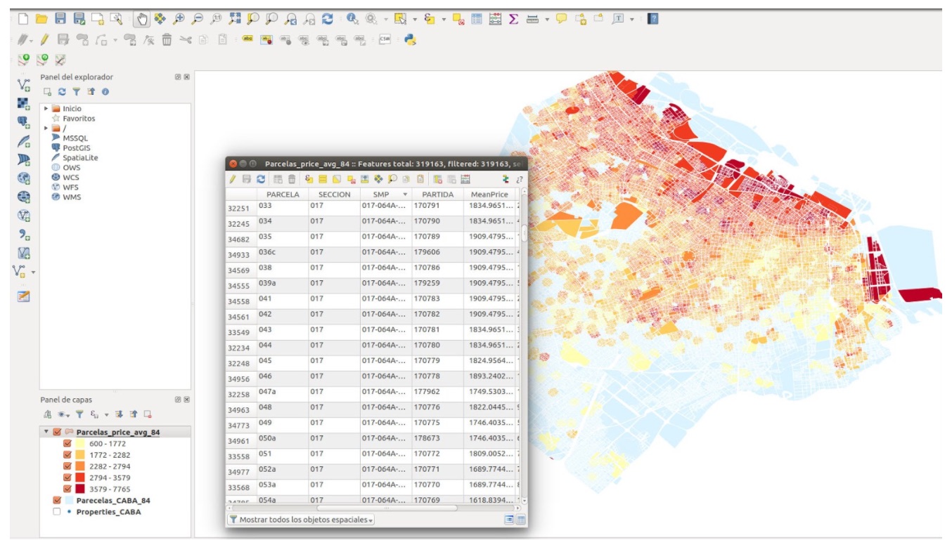
Calculate the price per square meter of every lot.
The average price per square meter corresponding to each lot is calculated using QGIS’s “spatial join” function with the datasets of properties and lots. Follow the link to this tutorial to see how to use the “spatial join” function.
We then join the data of the lots with the heights of each building. A merging of these datasets is executed by the lot names field.

Transform the shapefile into a vector tileset
Transform the shapefile into a vector tileset, which is a georeferenced information type that uses multiple digital mapping technologies to display the data. They are called “tilesets” because they are mosaic meshes that cover the desired surface; each mosaic has certain information that is being represented as we navigate a particular area of the map, or zoom in and out. Without these tilesets, displaying all the information that the map depicts would take too long.
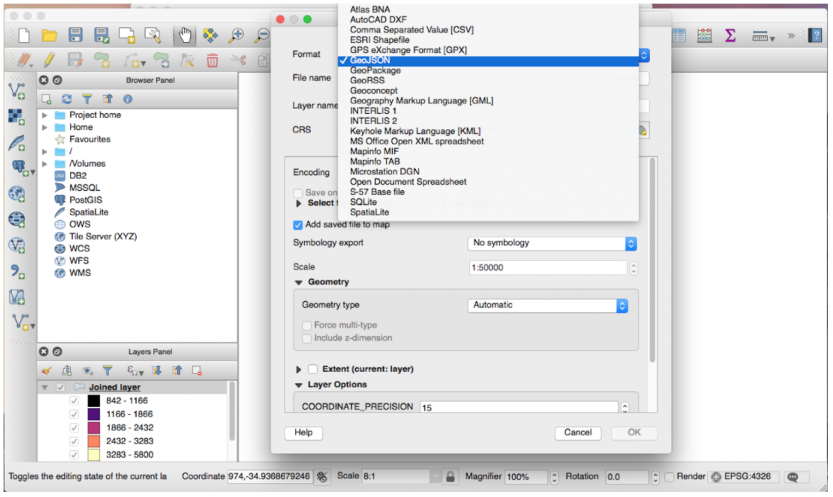
First, we must convert the shapefile from the first step to a GeoJSON.
(QGIS=> Save As => GeoJSON)
Upload the tileset to Mapbox
We’ll use Mapbox’s vector tile format, mbtiles, to upload our tileset. To convert GeoJSON to mbtiles, we will use the program tippecanoe.
tippecanoe -o 3d_map_tileset.mbtiles -z 17 -Z 12 3d_map_tileset.geojson
The z and Z parameters are important because the tilesets are constructed by zoom level. The wider the range of zooms used in the tileset, the larger the file.
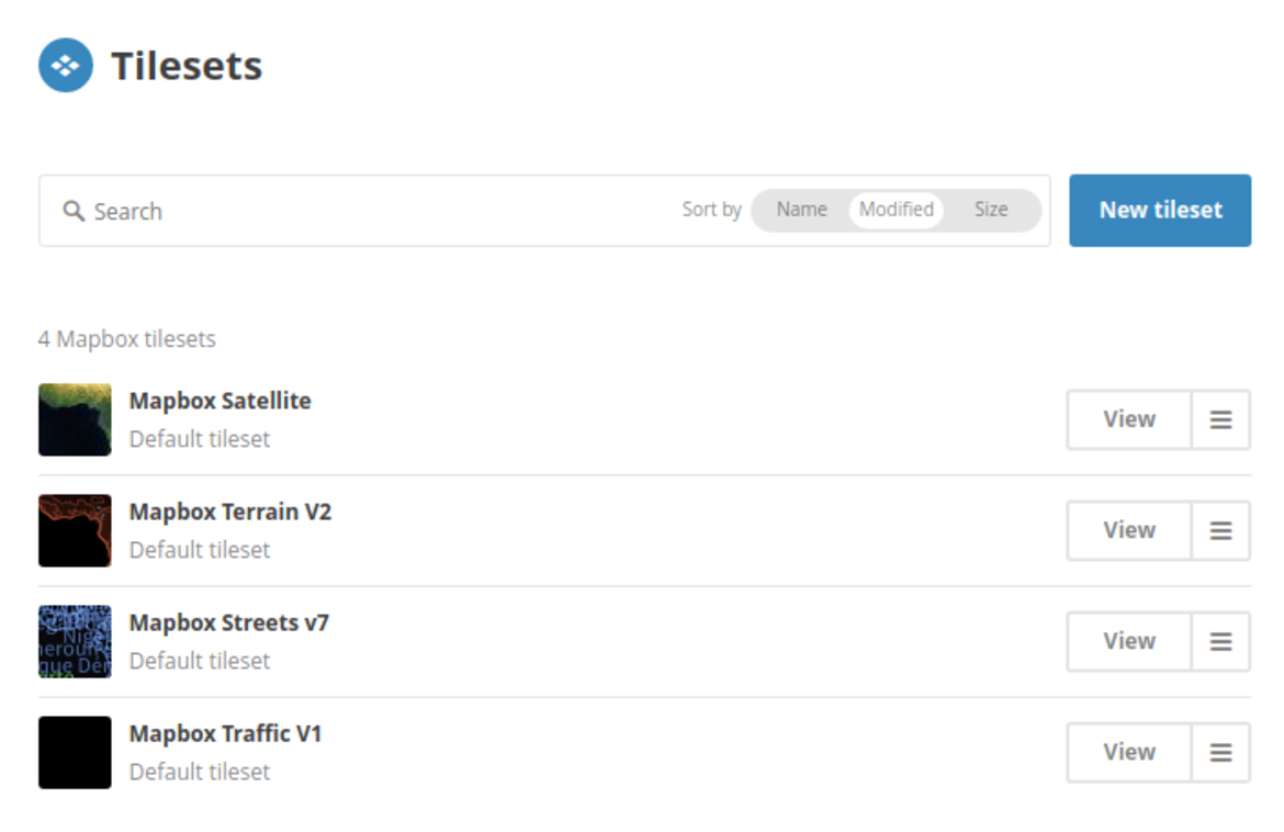
Once we’ve generated the file, we must upload it to the datasets section of Mapbox Studio.
Using Javascript to show the layers
We need to program some Javascript in order to show the layer. In fact, we have to make an application in Javascript that allows us to load both a base layer and the tileset at hand. To do so, we’ll use Mapbox GL JS. The API documentation can be found here.
Suppose we are going to do everything in a file named “our_map.html.”
Here are the necessary steps:
Create the html skeleton:
2. Load mapbox
3. Load the tileset:
Take note of these:
Here we are saying “take the heights of the buildings from the ‘altura’ field.”
Here we are saying “paint using the values in the ‘precio’ field, and use ranges to differentiate colors”: if there is no value, use ‘#e6e6e6’, if the value is between 0 and 700, use ‘#ffffb2’, if the value is between 700 and 1754, use ‘#fecc5c’. And so on.
The full code would be:
<html>

  <body

    <!-- mapbox gl js -->

    <script src='https://api.tiles.mapbox.com/mapbox-gl-js/v0.38.0/mapbox-gl.js'></script>

    <link href='https://api.tiles.mapbox.com/mapbox-gl-js/v0.38.0/mapbox-gl.css' rel='stylesheet' />

    <div style="padding:0; margin:0; width:100%; height:100%" id="map"></div>

    <script>

      window.onload = function(){

        var center = [-58.388875,-34.612427];


        mapboxgl.accessToken = 'YOUR ACCESS TOKEN';


        var map = new mapboxgl.Map({

          container: 'map',

          style: 'mapbox://styles/YOUTUSER/YOUR_BASE_STYLE',

          center: center,

          zoom: 13.5,

          pitch: 59.5,

          bearing: 0

        });


        map.on('style.load', function () {

          map.addSource('buildings',

              {"type": "vector",

                "url": "THE TILESET URL"

              });


          map.addLayer({

            'id': 'buildings',

            'interactive': true,

            'type': 'fill-extrusion',

            'source': 'buildings',

            'source-layer': 'super_new_join_finalgeojson',

            'paint': {

              'fill-extrusion-height': {

                'property': 'altura',

                'stops': [

                  [{zoom: 13, value: 0},   0],

                  [{zoom: 13.5, value: 1000}, 0],

                  [{zoom: 17.5, value: 0}, 0],

                  [{zoom: 17.5, value: 1000}, 1000]

                ]

              },

              'fill-extrusion-color': {

                'property': 'precio',

                'stops': [

                  [0, '#e6e6e6'],

                  [700, '#ffffb2'],

                  [1754, '#fecc5c'],

                  [2233, '#fd8d3c'],

                  [2751, '#f03b20'],

                  [3683, '#bd0026']

                ]

              },

              'fill-extrusion-opacity': 0.9

            }

          }, 'road_major_label');

        });

      }

    </script>

  </body>

</html>
Serve the HTML from a server
Now we must serve the html from a server. On our local machine we can use http-server, which can be installed with npm:
npm install http-server
Once installed, we must run it in the same folder as our html. Then, we navigate to localhost in the browser: 8080/our_map.html.
- How to build a 3D map of a city using QGIS and Mapbox - July 5, 2017