How to map point data and polygon shapefiles in R
I recently published a series of interactive maps for Beeradvocate magazine that explored storm surge scenarios and low-lying breweries in Boston, New York City, Charleston and Miami. Here’s Boston:
This is how I did it.
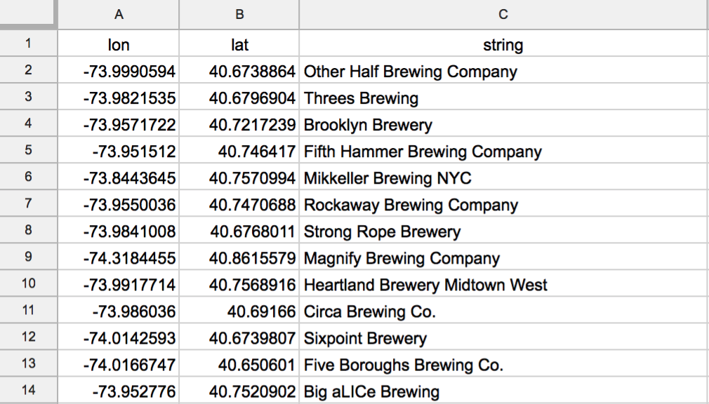
Getting lat, lon coordinates into a CSV
I first created CSV files for the four cities I was going to explore, amassing latitude and longitude coordinates and brewery names.
Download shapefiles from NOAA
The National Oceanic and Atmospheric Administration (NOAA) publishes shapefiles with various sea level rise scenarios on its website. I unzipped the files for my cities and brought all the gbdtable files into QGIS, an open-source mapping software.
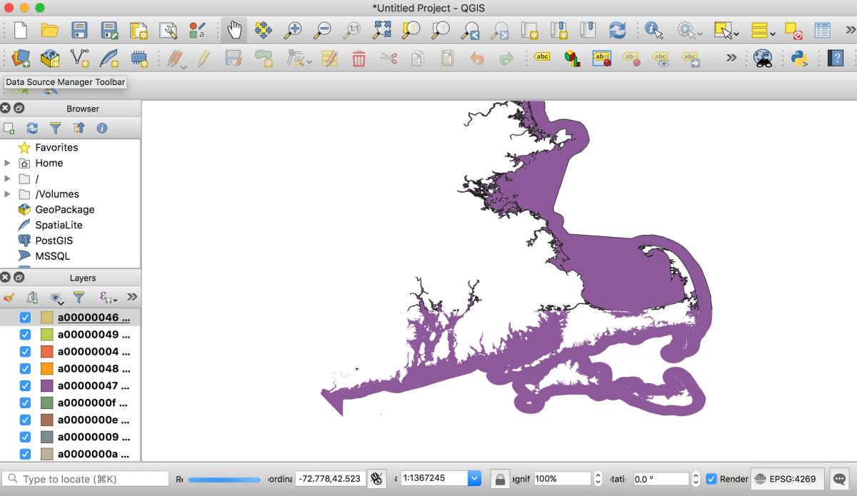
Then, I deselected every layer but the one ending in slr_8ft. With that layer selected, I went to Layer and hit Save As… and saved it as a geojson file. I did the same for every city I was exploring.
Why 8 feet? I was simulating Hurricane Sandy storm surge conditions which, when it hit New York, was measured at over 8 feet in some parts of Manhattan and New Jersey.
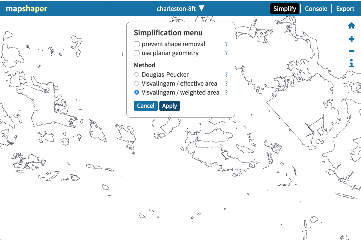
Simplifying your shapefiles so they’re not HUGE
Jeremy C.F. Lin, who just published a great analysis of sea level rise and Amtrak trains on Bloomberg, suggested I lower the weigh of my shapefiles using mapshaper.org. I dropped the geojson files and reduced the file size by 1/10th by clicking Simplify, then Apply for “Visvalingam/weighted area” and sliding the slider down to 1.5%. Then I exported new JSON files.
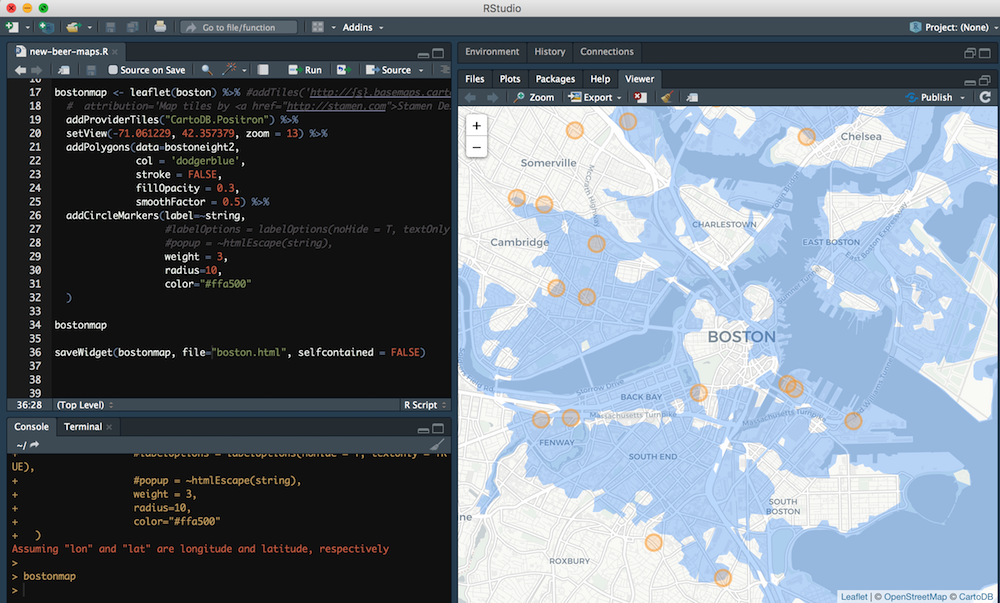
Bringing geojson files and CSVs into RStudio
Using the leaflet package in R, which has some decent documentation here, I brought my storm surge layer together with my point data. The geojsonio package smoothly brings in the geojson file.
library(tidyverse)
library(leaflet)
library(geojsonio)
library(htmlwidgets)
library(htmltools)

boston <- read.csv("bostonbrews.csv", stringsAsFactors=F)
bostoneight <- geojsonio::geojson_read("mass-8ft.json", what = "sp")

bostonmap <- leaflet(boston) %>%
  addProviderTiles("CartoDB.Positron") %>%
  setView(-71.061229, 42.357379, zoom = 13) %>%
  addPolygons(data=bostoneight,
              col = 'dodgerblue',
              stroke = FALSE,
              fillOpacity = 0.3,
              smoothFactor = 0.5) %>%
  addCircleMarkers(label=~string,
                   weight = 3,
                   radius=10,
                   color="#ffa500")
bostonmap
The final “bostonmap” will preview your map in RStudio’s plot window.
Styling basemap, markers and polygons
You can have fun styling the markers and polygons. As for the basemap, I’ve used the CartoDB Positron map for its simple design. More basemaps can be found here.
If you wish, you can add labels and a popup tooltip (with an X-out option) with the following code placed anywhere in the addCircleMarkers() section. (Beware overlapping labels – I haven’t been able to fix them! If anyone can inject this JS plugin into R, let me know.)
labelOptions = labelOptions(noHide = T, textOnly = TRUE),
popup = ~htmlEscape(string)
Exporting Leaflet map as HTML
Using the htmlwidgets package, I can export the map as an HTML file. Changing selfcontained to FALSE will put all ancillary files into a folder that exports with your HTML file.
saveWidget(bostonmap, file="boston.html", selfcontained = FALSE)Upload those files to your server and you’re done. Below, my finished maps.
Finished maps
Boston
New York City
Charleston
Miami


Very useful and instructive. Thanks a lot for sharing this. It helped me in building a Bus stop map for Bangalore, India