The explosion of AI data centers across the country this year has become a hot topic from small towns to the halls of Congress. That’s been reflected in the large number of stories published by local and national news organizations. We set out to analyze this intense media coverage and how the story around data centers is evolving over time, from the initial promises of economic growth with thousands of new jobs to the impacts suddenly being realized by local communities through increased resource usage leading to higher utility costs and environmental impacts. But reading through the thousands of news articles to identify these topics and get an accurate picture of the overall coverage seemed like an impossible task, so we found some ways to automate the heavy lifting. We’ll show you what we did — and how you can use similar methods to research other topics in media coverage.

For the analysis, we turned to Latent Dirichlet Allocation, or LDA, a topic modeling method that looks for words that appear together across documents. We wanted to see if it could help us spot patterns and make sense of a large collection of news coverage before digging into individual stories. Since all the articles in our dataset already mentioned data centers, the next question was what other topics appeared alongside them, for example energy and power, jobs, costs and taxes, local development and community concerns. LDA allowed us to look for these patterns across the full collection of articles.

But first, we needed to collect a library of news articles to analyze with LDA. We used Media Cloud, an open source platform for researching media, to search for news stories including the phrase “data center” from January through May 2026. Media Cloud gave us the titles of articles and their URLs, but not the article text, so we used newspaper4k, a Python script built for scraping web articles, for that part. Then we prepared the text for LDA and used the model to find and compare topics across the collection.

There were a few bumps along the way. Some websites block newspaper4k, and choosing the number of topics to search for took some testing. We’ll include those challenges, too, since they affected what we could actually do with the data.

Step 1: Import the packages needed to collect news articles

First, load the Python libraries we’ll need.Two packages are especially important at the start: mediacloud and newspaper4k. Media Cloud will help us find the articles. Newspaper4k will help us get the full text.

import itertools

import re

import datetime

import newspaper

import pandas as pd

import numpy as np

import networkx as nx

import matplotlib.pyplot as plt

from mediacloud.api import SearchApi

from sklearn.feature_extraction.text import CountVectorizer

from sklearn.model_selection import GridSearchCV

from sklearn.decomposition import LatentDirichletAllocation

Step 2: Find articles with Media Cloud

Using Media Cloud, we searched for “data center” and used January 1 through May 31, 2026 as our date range. Media Cloud returns information about the articles it has indexed, including their URLs, but it does not provide the full article text.

After registering an account with Media Cloud and getting a personal API key, the Media Cloud API allows us to quickly and easily perform this search by passing in a search string, datetime objects for our date range, and an ID for the media collection we would like to search.

start_date = datetime.date(2026, 1, 1)

end_date = datetime.date(2026, 6, 30)

MEDIACLOUD_KEY = "your_api_key_here"

US_NATIONAL_COLLECTION = 34412234

mc_search = SearchApi(MEDIACLOUD_KEY)

all_stories = []

pagination_token = None

more_stories = True

while more_stories:

   page, pagination_token = mc_search.story_list('"data center"', start_date=start_date, end_date=end_date, collection_ids=[US_NATIONAL_COLLECTION])

   all_stories += page

   more_stories = pagination_token is not None

print(f"Retrived {len(all_stories)} matching stories")

Step 3: Get the full text with newspaper4k

Now we have the article URLs from Media Cloud, but we still need the full text. This is where newspaper4k comes in. This package allows us to scrape articles from the URLs we got in the last step.

Some websites use Cloudflare or similar services to block scrapers like this, so we exclude them when the text cannot be retrieved to speed up the scraping process.

blocked = []

for index, row in df.iterrows():

   if row["media_name"] not in blocked:

       try:

           article = newspaper.article(row["url"])

       except Exception as e:

           print(str(e))

           if "protected with PerimeterX" in str(e):

               blocked.append(row["media_name"])

           elif "protected with Cloudflare" in str(e):

               blocked.append(row["media_name"])

           elif "protected with CloudFront" in str(e):

               blocked.append(row["media_name"])

           continue

       df.at[index, "text"] = article.text

Step 4: Preprocess the text

Now that we have the full article text, we need to prepare it for the analysis. We start with some standard preprocessing: converting all text to lowercase and removing non-alphanumeric characters and numbers.

def preprocess(s):

   s = s.lower()               # set to lower case

   s = re.sub(r'\W', ' ', s)   # remove any non alphanumeric characters

   s = re.sub(r'\d', ' ', s)   # remove numbers

   return s

df["preprocessed"] = df["text"].apply(preprocess)

The cleaned text is then saved in a new preprocessed column.

Step 5: Remove stopwords

Next, we remove stopwords,  common words that are not very helpful for identifying topics. We use NLTK’s stopword list and add a few extra words specific to our data. The code then uses CountVectorizer to turn the preprocessed text into word counts for the LDA model, skipping words in the stopword list and those which occur in fewer than 10% or more than 90% of the documents.

stop_words = [

   "i", "me", "my", "myself", "we", "our", "ours", "ourselves", "you", "your", "yours", "yourself", "yourselves",

   "he", "him", "his", "himself", "she", "her", "hers", "herself", "it", "its", "itself", "they", "them", "their", "theirs", "themselves",

   "what", "which", "who", "whom", "this", "that", "these", "those",

   "am", "is", "are", "was", "were", "be", "been", "being", "have", "has", "had", "having", "do", "does", "did", "doing",

   "a", "an", "the", "and", "but", "if", "or", "because", "as",

   "until", "while", "of", "at", "by", "for", "with", "about", "against", "between", "into", "through", "during", "before", "after", "above", "below", "to", "from",

   "up", "down", "in", "out", "on", "off", "over", "under", "again", "further",

   "then", "once", "here", "there", "when", "where", "why", "how", "all", "any", "both", "each", "few", "more", "most", "other", "some", "such",

   "no", "nor", "not", "only", "own", "same", "so", "than", "too", "very", "s", "t", "can", "will", "just", "don", "should", "now"

] + ["said", "mr"] + ["article", "continues", "below", "this", "ad", "advertisement"]

vectorizer = CountVectorizer(stop_words=stop_words, min_df=0.1, max_df=0.90)

tf = vectorizer.fit_transform(df["preprocessed"])

Step 6: Choose the number of topics

Now we’re ready to run LDA. LDA comes down to a simple idea: a document is made up of a set of topics, topics are made up of a set of words, and there are probability distributions which can be calculated to define these.  However, these distributions will look different for different corpera, so we need to adjust several parameters to account for that.

The number of topics is a parameter which tends to produce the largest effect when it’s changed, so we start with this variable.

To do this, we ran the model with default parameters while only adjusting the number of topics between iterations and then computing the log likelihood for the resultant word and topic distributions. This continuously gets better as the number of topics increases, but eventually hits a point of diminishing returns. LDA’s best performance is around this cusp, and identifying the number of topics in this way is often referred to as the “elbow method.” Using the number of topics in this range allows us to run fewer iterations of the model as we fine tune other variables, which affords us significant time savings.

scores = []

for n_topics in list(range(14, 21, 2)):

   lda = LatentDirichletAllocation(

       n_components=n_topics,

       random_state=867

   )

   lda_output = lda.fit_transform(tf)

   print(lda.perplexity(tf))

   scores.append(lda.perplexity(tf))

plt.plot(list(range(6, 25)), scores)

plt.xticks(list(range(6, 25)))

plt.xlabel("# topics")

plt.ylabel("perplexity")

plt.show()

Step 7: Adjusting hyperparameters

Once we have the number of topics, the next step is to tune the document-topic and topic-word priors so that EXPLAIN WHY IT’S NECESSARY TO TUNE. These settings affect how topics are distributed across documents and how words are distributed across topics. 

In our case, news articles tend to focus on a single topic, like the government or the economy, so a lower document-topic prior works best. This helps the model to not split topics up.

Words, on the other hand, are more likely to be used across a variety of topics, such as how “energy” is discussed with respect to its generation, distribution, or costs, and how “bill” may refer to a piece of legislation or the cost of something, so a higher topic-word prior works best here. This prevents the model from combining topics which otherwise should be separate, but happen to share some words in common.

We can verify that these make sense by running this model a couple times with high, medium, and low values for these parameters, but there are lots of combinations to check so we automate this using a grid search.

Step 8: Fine tuning with grid search

Since we now have an idea of about how many topics will be identified and what the topic-word and document-topic priors should be, we can start fine tuning each of those parameters.

The idea of grid search is trying every combination of several different values for each of the variables we’re adjusting, and then seeing which ones work the best. Because the number of combinations scales with the power of the number of variables (adding one variable with two values doubles the number of runs) this can end up needing to run many times, which is why we got ourselves into a general range with the previous steps.

param_grid = {

   "n_components": range(14, 15),

   "doc_topic_prior": [0.1, 0.25, 0.4],

   "topic_word_prior": [0.6, 0.75, 0.9],

}

lda = LatentDirichletAllocation(random_state=867)

cv = GridSearchCV(estimator=lda, param_grid=param_grid, n_jobs=8)

cv.fit(tf)

Step 9: Check the topics manually

The number of times a topic occurs is not the only thing we look at. We also check the topics ourselves. For this step, we look at the groups of words produced by the model and ask a simple question: Do these word groupings make sense based on what we have seen in the articles?

def plot_top_words(model, feature_names, n_top_words, title):

   fig, axes = plt.subplots(4, 5, figsize=(30, 25), sharex=True)

   axes = axes.flatten()

   for topic_idx, topic in enumerate(model.components_):

       top_features_ind = topic.argsort()[-n_top_words:]

       top_features = feature_names[top_features_ind]

       weights = topic[top_features_ind]

       ax = axes[topic_idx]

       ax.barh(top_features, weights, height=0.7)

       ax.set_title(f"Topic {topic_idx}", fontdict={"fontsize": 30})

       ax.tick_params(axis="both", which="major", labelsize=20)

       for i in "top right left".split():

           ax.spines[i].set_visible(False)

       fig.suptitle(title, fontsize=40)

   plt.subplots_adjust(top=0.90, bottom=0.05, wspace=0.90, hspace=0.3)

   plt.show()

plot_top_words(lda, vectorizer.get_feature_names_out(), 10, "LDA")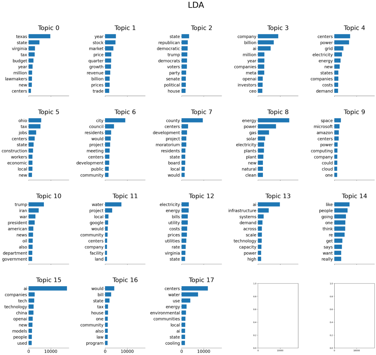

Each chart shows one topic and the words associated with it. This gives us a way to check whether the topics produced by the model are actually meaningful before moving on to the article-level analysis.

Step 10: Add topic labels to the articles

After checking that the topics make sense, the next step is to add the topic labels back to the articles.

Since LDA calculates the probabilities of the word and topic distributions across all articles, we can essentially just use it in reverse to find the probability distribution of topics in an article. Assigning the topic with the highest probability to an article lets us see if there is any difference in the number of articles covering each topic by region and over time.

def get_top_words(lda, topic, vectorizer, n_words):

   return vectorizer.get_feature_names_out()[lda.components_.argsort()[topic][-n_words:]][::-1]

# Get dominant topic and top words for each document

df["dominant_topic"] = lda_output.argmax(axis=1)

# Add top words to help keep track of topics

topic_dict = {topic: f", ".join(get_top_words(lda, topic, vectorizer, 5)) for topic in df["dominant_topic"].unique()}

df["top_words"] = df["dominant_topic"].map(topic_dict)

# Add all topic probabilities

for i in range(n_topics):

   df[f"topic_{i}_prob"] = lda_output[:, i]

Step 11: Plot the topic distributions

Finally, we can plot the topics to see how they are distributed across different parts of our dataset. For our project, we compared national coverage with coverage from Ohio, Virginia and Texas.

fig, axs = plt.subplots(2, 2, figsize=(12, 12), sharey=True)

idxs = itertools.product([0, 1], [0, 1])

regions = ["national", "ohio", "virginia", "texas"]

topics = list(range(0, 14))

for region, idx in zip(regions, idxs):

   df[df["location"] == region]["dominant_topic"].value_counts().reindex(topics).plot.barh(ax=axs[idx])

   axs[idx].set_title(region)

   axs[idx].set_xlabel("# articles")

   axs[idx].set_yticklabels([", ".join(get_top_words(lda, topic, vectorizer, 5)) for topic in topics])

fig.tight_layout()

plt.show()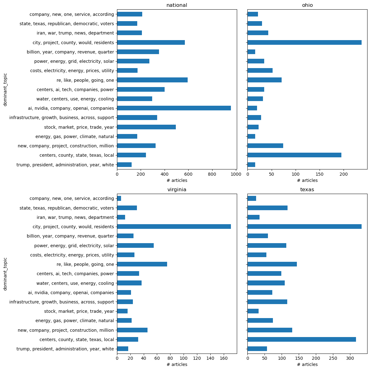

Each chart shows the number of articles for each topic in that part of the dataset.

Why this workflow matters

News coverage can add up quickly. A few months of reporting on one issue can mean hundreds or thousands of articles, which makes it hard to see what the coverage looks like as a whole. LDA gives us one way to zoom out and find topics across all of those stories at once.

For journalists working with large collections of news articles, this approach makes it possible to move from thousands of individual stories to a set of topics that can actually be compared. Once the articles have topic labels, they can be grouped by location, outlet or time period to look for differences in coverage. The same process can be reused with a different Media Cloud search, making it a starting point for other reporting questions rather than a one-time analysis.

Other thoughts

The automation made possible with this method is powerful, but it is still important to read through some amount of the corpus and gain familiarity with the texts being worked on before running it.  Actually reading some articles helped us to find appropriate stop words; for example, the sentence “article continues after ad” appeared in about 20% of the articles scraped.  It also allowed us to confirm that “energy” showing up in four somewhat overlapping, but still distinct, topics made sense.