A Data History of Popular Hip-Hop
By Alexander Frandsen
Hip-hop has come a long way from the days of the Sugarhill Gang and Kurtis Blow. According to Nielsen Music’s 2017 year-end report, hip-hop has officially overtaken rock as the most popular genre in the country, and it is nearly impossible to peruse radio stations these days without hearing Drake or Migos.
Hip-hop has simply become a centerpiece of American culture. When Childish Gambino dropped “This is America” this past May, for instance, outlets like The Atlantic and The Washington Post dedicated a significant amount of coverage to the song, dissecting every possible metaphor and hidden meaning. When Kanye West makes a controversial statement, it’s covered by CNN and Complex alike.
But for all the increased attention paid to hip-hop, most analysis of the genre is done qualitatively. Discussions of its themes and content are mostly relegated to think pieces and opinion-heavy feature stories.
Of course, that’s natural for coverage of any art form. But as you know, we here at Storybench are all about the data. So we looked at the past 30 years of popular hip-hop and broke it down quantitatively. We used Billboard’s “Hot Rap Songs” category to create our dataset, and scraped Genius’s API to get all the lyrics for each entry. (For a detailed look at how we did, check out this tutorial).
It’s an imperfect dataset, to be sure. Even though rap was starting to assert itself in the 1980’s, Billboard only established the “Hot Rap Songs” category in 1989, so we’re missing a good decade. But given that rap mostly entered the mainstream in the 1990’s, it should still give us a good sense of how the genre has changed – or stayed the same – over time. Off we go!
How did hip-hop spread geographically?
Hip-hop is now obviously a national entity, but it certainly wasn’t always that way. Many of the most well-known artists in rap’s early days of popularity hailed from a few select areas. To figure out how the genre’s grown geographically, we popped our data into Carto and plotted where each chart-topping rapper was from. Here’s the map animated over time.
The map evolves pretty logically. New York City is the historic home of rap going back to the days of Bronx block parties, and the map shows not only how many popular artists are from the Big Apple, but also how the genre began to creep up and down the East Coast from there. Contemporary epicenters like southern California, south Florida, and Houston emerge early on as well. As the 1990’s bled into the 2000’s, rappers like Nelly and Kanye West helped put Midwestern cities like Chicago and St. Louis on the map. By the time we hit the 2010’s, mainstream rap is coming from nearly every corner of the country. There’s a notable gap in the middle of the map, though: Between the Mississippi River and the West Coast, there are nearly no Billboard-charting rappers outside of Texas.
Historical text analysis
Now we know how popular hip-hop has spread geographically. But what about the actual content? To get into the lyrical side of things, we booted up R and dove into the “tidytext” package, essentially a method that breaks down chunks of text into individual “tokens” that serve as data points for analysis. This guide from its creators, Julia Silge and David Robinson, is immensely helpful in learning the basics.
You can find the full code on Github, but we’ll also include some of it here for important steps.
Most used words across all years
The first analysis we did was simple: What words have been used the most in popular hip-hop? This isn’t perfect, but it should at least let us know what themes have dominated songs. After filtering out curse words, stop words, and meaningless terms like “yo” and “hey,” these are the results:
tidy_lyrics %>%
  count(word, sort = TRUE)
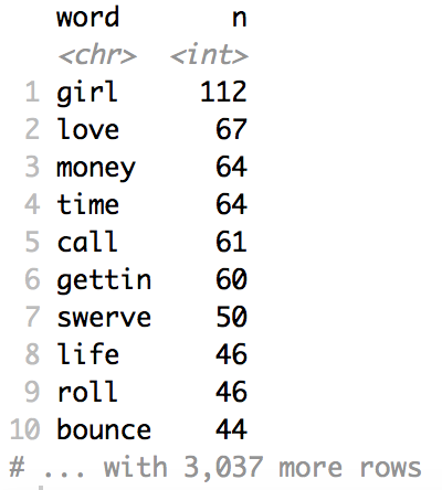
For a genre that gets accused of encouraging violence, this is a pretty positive list! Romance is the most popular topic of discussion, and universal worries like wealth and time are reflected, too. Hip-hop has been siloed as a “street thing” for much of its existence, but this shows that it’s simply a human thing.
Unique words by decade
But let’s get a little more complex. Are there certain words and themes that stick out for each decade? Instead of doing a simple count, we’ll use a technique called tf-idf (or term frequency inverse document frequency and outlined here) to pull out unique words. The idea is that you get rid of commonly used words and instead pull out words that are distinct within a category compared to the rest of the dataset.
tf_idf_words <- tidy_lyrics %>%
  count(word, decade, sort = TRUE) %>%
  bind_tf_idf(word, decade, n) %>%
  arrange(desc(tf_idf))

glimpse(tf_idf_words)

top_tf_idf_words <- tf_idf_words %>%
  group_by(decade) %>%
  filter(!decade == "1980s") %>%
  top_n(12) %>%
  ungroup()

ggplot(top_tf_idf_words, aes(x = reorder(word, n), y = n, fill = decade)) +
  geom_col(show.legend = FALSE) +
  facet_wrap(~decade, scales = "free") +
  coord_flip()
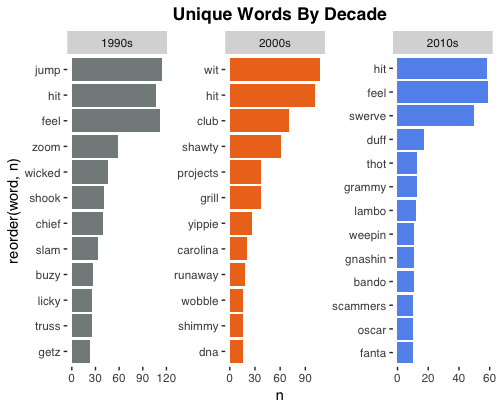
It’s a little rough around the edges, but some generational differences definitely start to emerge. Words like “bando,” “swerve,” and “fanta” are prominent in the current decade of hit rap songs, which makes a lot of sense given the immense popularity of trap. (In case you need a translation: “bando”=an abandoned house, “swerve”=get out of the way, and “fanta” usually refers to using the soda as an ingredient in making lean.)
The 2000’s popular rap scene was heavier on club bangers, which is shown in the prevalence of “shimmy,” “wobble,” and “club.” The words for the 1990’s are a little less revealing, but “hit,” “shook,” and “slam” seem to point towards the popularity of gangsta rap at the time.
Lyrical complexity over time
We are in the midst of the “mumble rap” era, which has mostly been defined by rappers like Young Thug, Future, and Lil Uzi Vert. Lyricism seems to have fallen to the wayside a bit, and there has been much discussion over whether rap is getting “dumber.” But is that really the case? If we look at lyrical complexity for our hit rap songs over the years, we might be able to test that hypothesis. Of course, since our dataset is limited to Billboard charting songs, we’re only getting a sense of the complexity of popular songs, but that should still give us an idea of what the mainstream rap crowd has had an appetite for. We’ll omit the 1980’s again due to the lack of data.
word_summary <- tidy_lyrics %>%
  group_by(decade, Song) %>%
  filter(!decade == "1980s") %>%
  mutate(word_count = n_distinct(word)) %>%
  select(Song, Released = decade, word_count) %>%
  distinct() %>% #To obtain one record per song
  ungroup()

install.packages("yarrr")
library(yarrr)
pirateplot(formula =  word_count ~ Released, #Formula
           data = word_summary, #Data frame
           xlab = NULL, ylab = "Song Distinct Word Count", #Axis labels
           main = "Lexical Diversity Per Decade", #Plot title
           pal = "google", #Color scheme
           point.o = .2, #Points
           avg.line.o = 1, #Turn on the Average/Mean line
           theme = 0, #Theme
           point.pch = 16, #Point `pch` type
           point.cex = 1.5, #Point size
           jitter.val = .1, #Turn on jitter to see the songs better
cex.lab = .9, cex.names = .7) #Axis label size 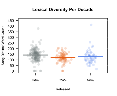
It’s not terribly conclusive, but there might be some credence to the theory that rap is getting simpler. The median complexity of the 1990’s sits the highest of any decade, which could justify the old heads who lament the days of 2pac and Biggie. But the difference is fairly slight, and the 2000’s were actually a little less complex than the 2010’s, which could redeem the mumble rap era.
Regional text analysis
We’ve used text analysis to look for historical differences, but what about geographic ones? More so than other genres, rap takes great pride in its distinct regional personalities, so it makes sense to check out whether different regions are noticeably different in their lyricism. Since regional tastes are often defined by more lower-level artists, these analyses should be taken with a grain of salt, but hopefully we can still pull out some unique traits.
Unique words by region
Let’s use tf-idf again to pull out regional favorites.
glimpse(tidy_lyrics)

tf_idf_words2 <- tidy_lyrics %>%
  count(word, Region, sort = TRUE) %>%
  bind_tf_idf(word, Region, n) %>%
  arrange(desc(tf_idf))

glimpse(tf_idf_words2)

top_tf_idf_words2 <- tf_idf_words2 %>%
  group_by(Region) %>%
  filter(!Region == "NA") %>%
  top_n(12) %>%
  ungroup()

ggplot(top_tf_idf_words2, aes(x = reorder(word, n), y = n, fill = Region)) +
  geom_col(show.legend = FALSE) +
  facet_wrap(~Region, scales = "free") +
  coord_flip()
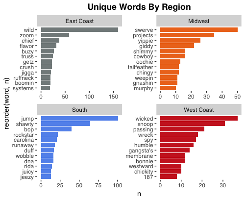
Again, it’s a little messy, but some obvious points jump off the graphs. Chicago’s own Kanye West largely popularized the term “swerve,” so it makes sense that it is tied so strongly to the Midwest. “Wicked,” “wreck,” and “gangsta’s” stick out for the West Coast, which could be explained by the gangsta rap wave headed by California-based rappers like Coolio and 2pac in the 1990’s and early 2000’s. “Shawty” is a distinctly southern word that’s entered the mainstream hip-hop lexicon, but its rank on the list is a good reminder of where the term actually came from. The East Coast is a little harder to make sense of, but Jay-Z’s dominance over the New York scene shines through with the word “jigga.”
Complexity by region
Now let’s go back to lyrical complexity, and see whether some regions pick up the dictionary and thesaurus a little more than others.
word_summary <- tidy_lyrics %>%
group_by(Region, Song) %>%
filter(!Region == "NA") %>%
mutate(word_count = n_distinct(word)) %>%
select(Song, Region = Region, word_count) %>%
distinct() %>% #To obtain one record per song
ungroup()pirateplot(formula = word_count ~ Region, #Formula
data = word_summary, #Data frame
xlab = NULL, ylab = "Song Distinct Word Count", #Axis labels
main = "Regional Lexical Diversity", #Plot title
pal = my.color, #Color scheme
point.o = .2, #Points
avg.line.o = 1, #Turn on the Average/Mean line
theme = 0, #Theme
point.pch = 16, #Point `pch` type
point.cex = 1.5, #Point size
jitter.val = .1, #Turn on jitter to see the songs better
cex.lab = .9, cex.names = .7) #Axis label size
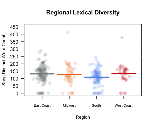
At least among Billboard-charting rap songs, the race is pretty tight. The East Coast, West Coast, and Midwest are all essentially even, and the South is a close but clear fourth. Given that trap music came from the South and is known for its simple hooks and repetitive lyrics, this makes some sense. But it’s safe to say, given the narrow spread of the data, that we can’t make a real conclusion about which region flexes their vocabulary the most.
Some (rudimentary) sentiment analysis
Hip-hop is deeply rooted in emotion, so we would be remiss to ignore sentiment analysis. There are a few lexicon emotion libraries available on R, but we’ll use “bing,” which is helpful because it sorts words into a positive/negative binary.
tidy_lyrics %>%
  inner_join(get_sentiments("bing")) %>%
  count(sentiment) %>%
  spread(sentiment, n, fill = 0) %>%
  mutate(sentiment = positive - negative)

This shows us that mainstream rap songs have had more negative lyrics than positive ones. The genre as a whole is deeply rooted in the black struggle, so perhaps this shouldn’t come as a surprise. But if this indicates that the majority of rap lyrics are negative, has that level of negativity changed over time? Let’s look at sentiment polarity over time to get a sense. R simply subtracts negative word count from positive word count to find this for each year.
lyrics_polarity_year <- lyrics_bing %>% count(sentiment, Year) %>% spread(sentiment, n, fill = 0) %>% mutate(polarity = positive - negative, percent_positive = positive / (positive + negative) * 100)polarity_over_time <- lyrics_polarity_year %>% ggplot(aes(Year, polarity, color = ifelse(polarity >= 0,my_colors[5],my_colors[4]))) + geom_col() + geom_smooth(method = "loess", se = FALSE) + geom_smooth(method = "lm", se = FALSE, aes(color = my_colors[1])) + theme_lyrics() + theme(plot.title = element_text(size = 11)) + xlab(NULL) + ylab(NULL) + ggtitle("Polarity Over Time")relative_polarity_over_time <- lyrics_polarity_year %>% ggplot(aes(Year, percent_positive , color = ifelse(polarity >= 0,my_colors[5],my_colors[4]))) + geom_col() + geom_smooth(method = "loess", se = FALSE) + geom_smooth(method = "lm", se = FALSE, aes(color = my_colors[1])) + theme_lyrics() + theme(plot.title = element_text(size = 11)) + xlab(NULL) + ylab(NULL) + ggtitle("Percent Positive Over Time")
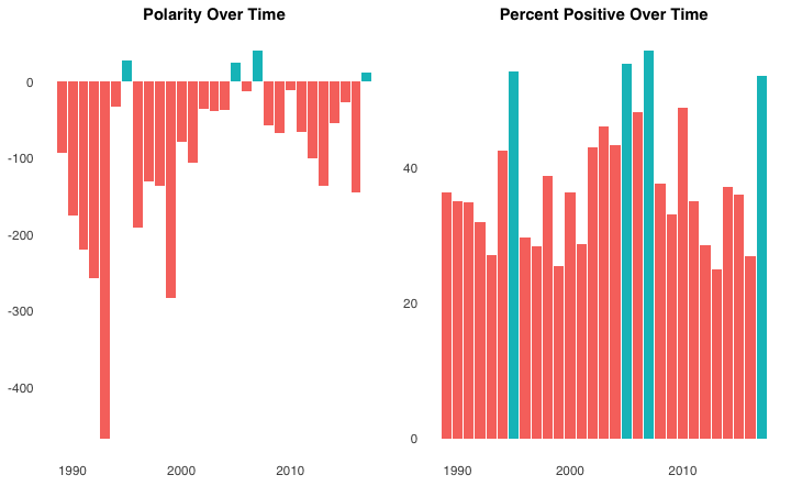
We made graphs for both overall polarity over time and for the percent of words that are positive over time. The first is useful to show just how dominant negativity has been in rap over the years, but the second is a bit more straightforward and easier to read.
The obvious trend is that rap has become slightly more positive. It’s impossible to isolate a clear explanation for this, but a possibility is that as rap has become more mainstream over time, its popular songs have gravitated away from core hip-hop themes, like racism and crime, to more universally palatable ones, like wealth and success.
The spikes are interesting to note as well. The most drastic one in the first graph is in 1993, which stretches all the way past -400. If we take a look at what was going on in the U.S. around that time, one event sticks out—the Rodney King riots. The riots decimated L.A. (a noted rap hub) in 1992 and served as a boiling-over point for race relations in the country. Given the natural gap between a song’s thematic inspiration and its eventual release, it seems quite possible that the negative spike we see in 1993 is a reaction to the racially-charged events of 1992.


