If you have ever opened the U.S. Census website looking for tract-level data, you know how quickly things can get overwhelming. Tables, codes, geographies, shapefiles, downloads: before you even ask a question, you are already having to decide which tools you need to answer it.

Inspired by a video explainer by Kyle Walker, this  tutorial starts from a simpler place: a blank project in Positron and a single question. How quickly can you go from raw Census data to a usable map using R?

Using the tidycensus package, I pulled American Community Survey data at the census tract level, letting R handle both the data and the geography in one step. Instead of manually downloading shapefiles or opening a GIS interface, tract boundaries are included directly by setting geometry = TRUE. The result is a single spatial data object that can be inspected, mapped, and reused.

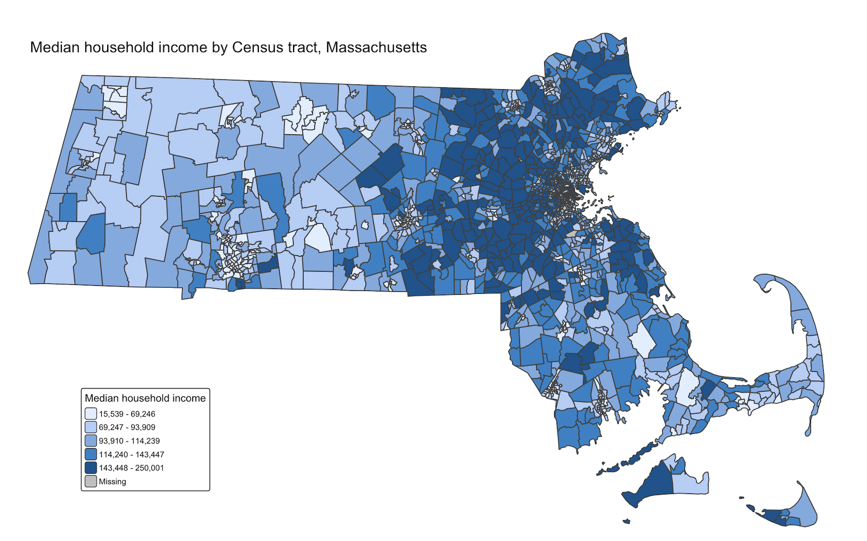
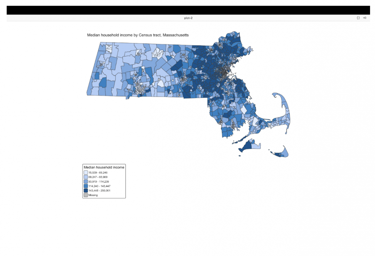
To make the process concrete, I mapped median household income across Massachusetts Census tracts. The goal was not to design a polished visualization, but to understand the workflow: authenticating with the Census API, requesting tract-level data, confirming what the data actually contains, and rendering a basic choropleth map using tmap.

Throughout the process, I documented each step with screenshots, including moments where things did not immediately work as expected. That friction is part of the story. Restarting the R session after registering an API key, understanding where exported files are saved, and recognizing how spatial objects behave in R are all small details that matter when you are new to this workflow.

Census tract data is a common foundation for local reporting on housing, inequality, language access, and public health. This walkthrough shows one way to make that data feel more approachable by keeping the pipeline short, transparent, and reproducible. Once the data is in this form, it can just as easily be exported for web mapping, combined with other datasets, or extended into a more interactive project.

What you’ll need

• R installed on your machine
• Positron or another notebook installed
• A free Census API key
• About 10 minutes

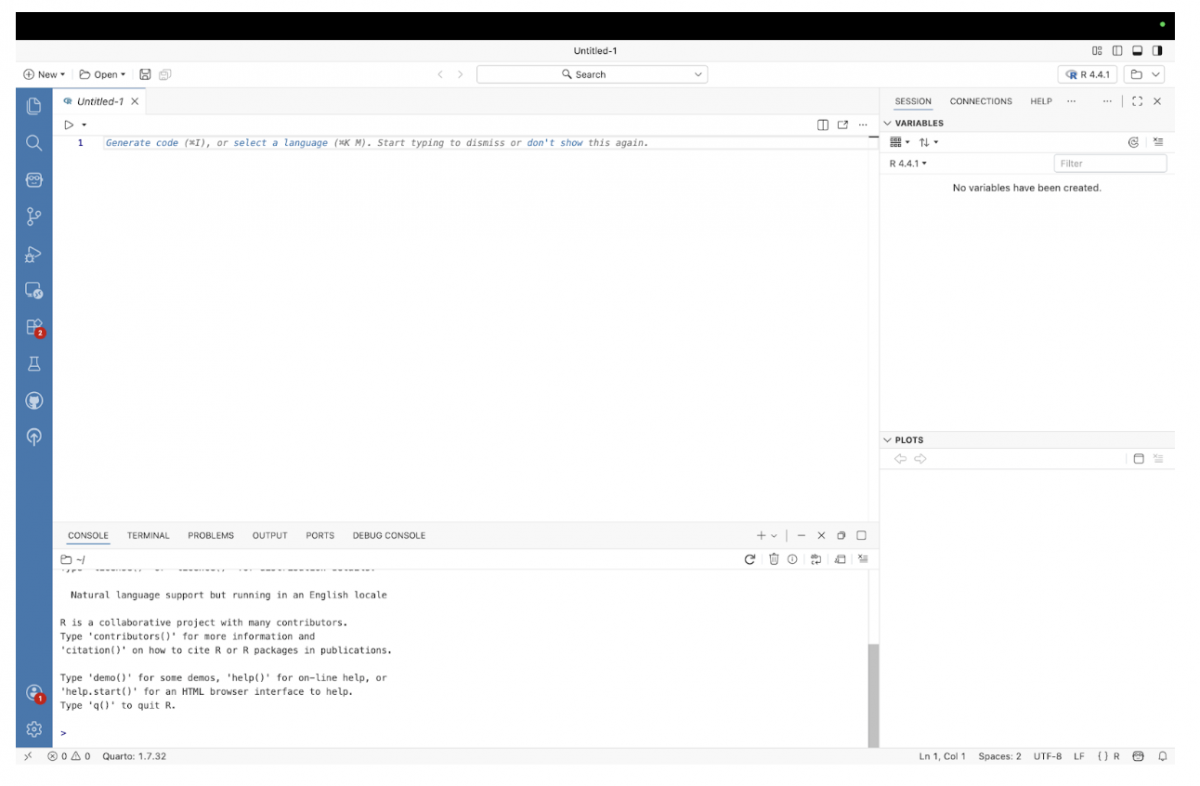
Step 1: Install R and open Positron

If you haven’t already, install R from the official R website. Once installed, open Positron and create a new R script. Positron works much like VS Code or other code editors with previews, but is especially useful  for R and Python workflows.

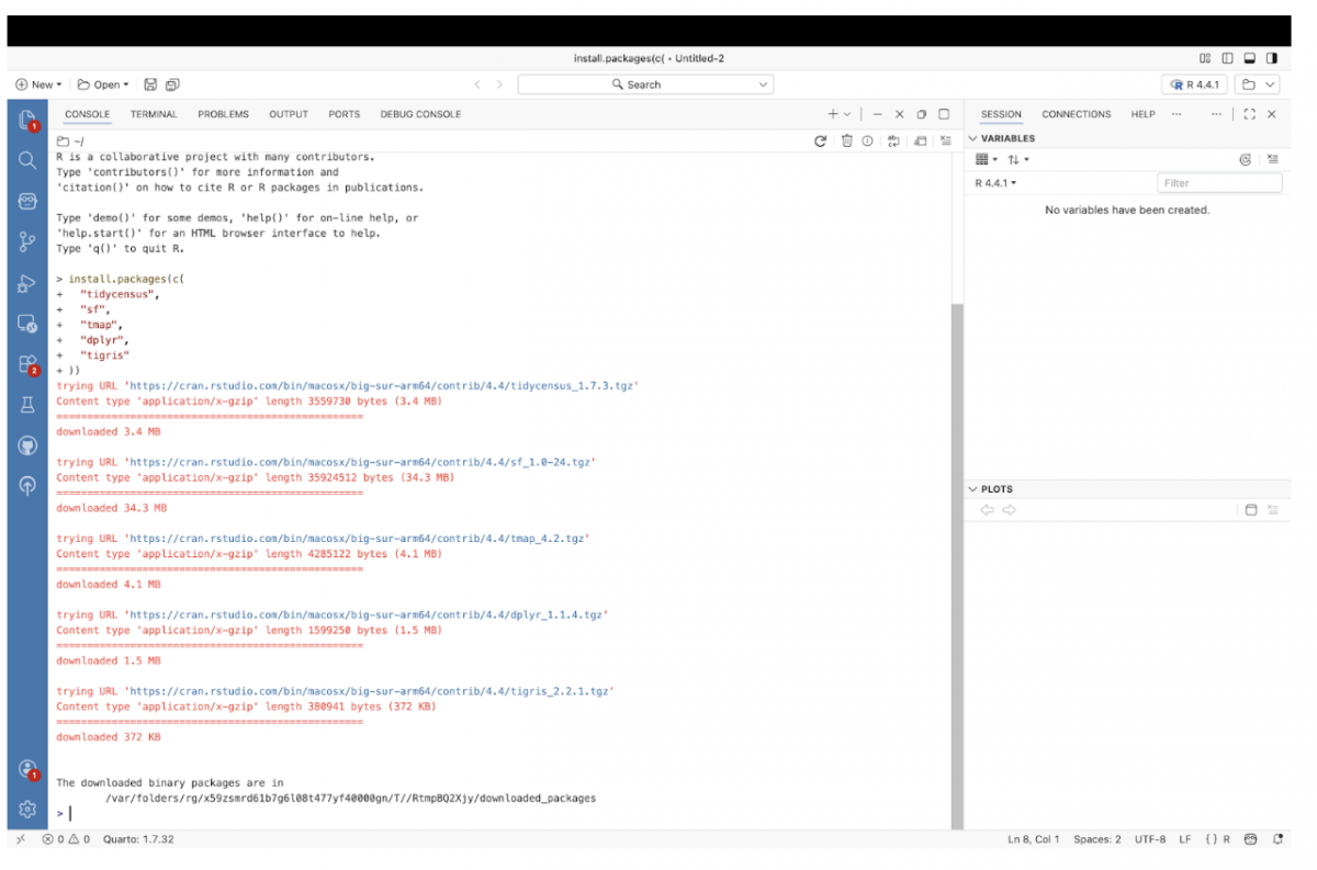
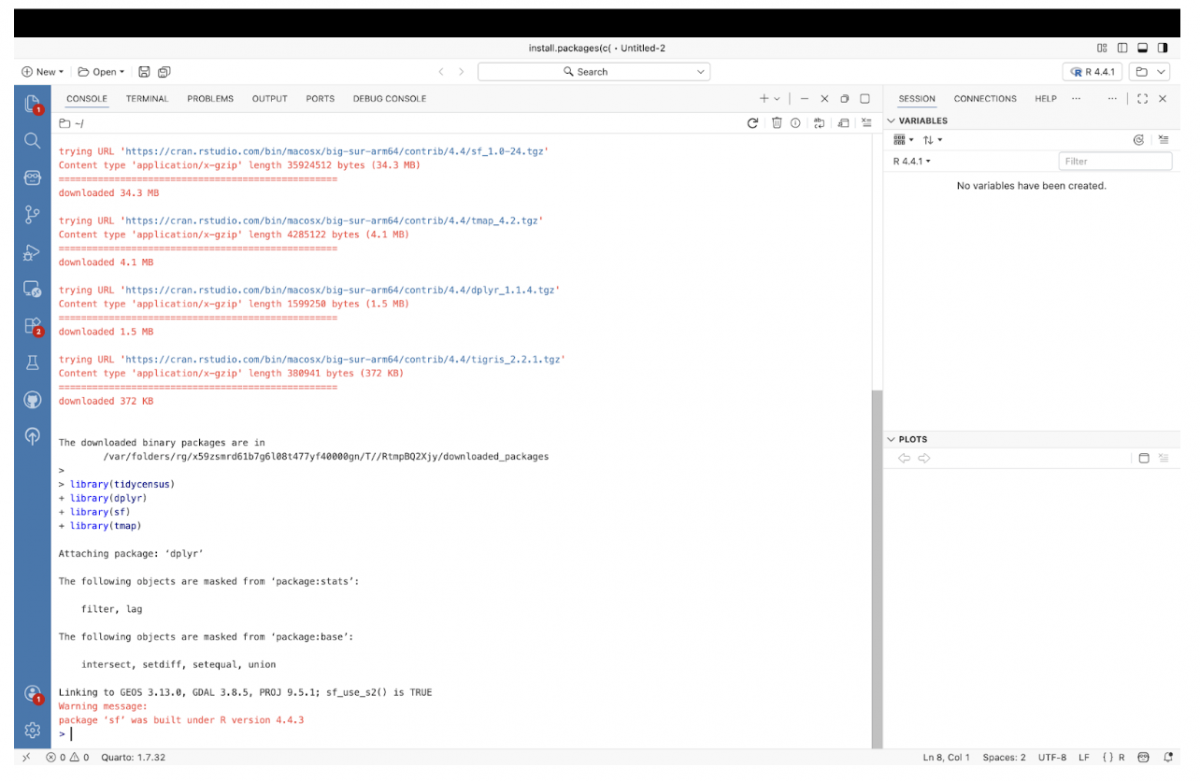
Step 2: Install the required packages

In the Console, install the packages needed to pull Census data and create a map.

install.packages(c(
  "tidycensus",
  "sf",
  "tmap",
  "dplyr",
  "tigris"
))

This only needs to be done once.

Step 3: Load the libraries

After installation, load the libraries into your R session.

library(tidycensus)
library(dplyr)
library(sf)
library(tmap)

If you don’t see any error messages, you’re ready to go.

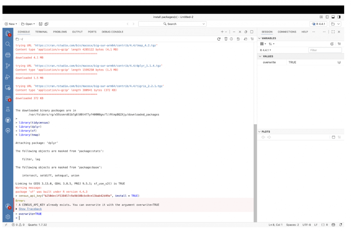
Step 4: Request a Census API key

To access American Community Survey data, you’ll need a free Census API key. You can request one from the U.S. Census Bureau’s API signup page. The key is emailed almost immediately.

Once you have the key, register it in R:

census_api_key("YOUR_API_KEY_HERE", install = TRUE)

Restart your R session after running this so the key takes effect.

Step 5: Restarting R means reloading libraries

After restarting R, all previously loaded libraries are cleared. This is a common point of confusion.

Before doing anything else, load the libraries again:

library(tidycensus)
library(dplyr)
library(sf)
library(tmap)

If this step is skipped, R will not recognize functions like get_acs().

Step 6: Cache Census geography

Tell R to cache Census boundary files so they do not need to be downloaded repeatedly.

options(tigris_use_cache = TRUE)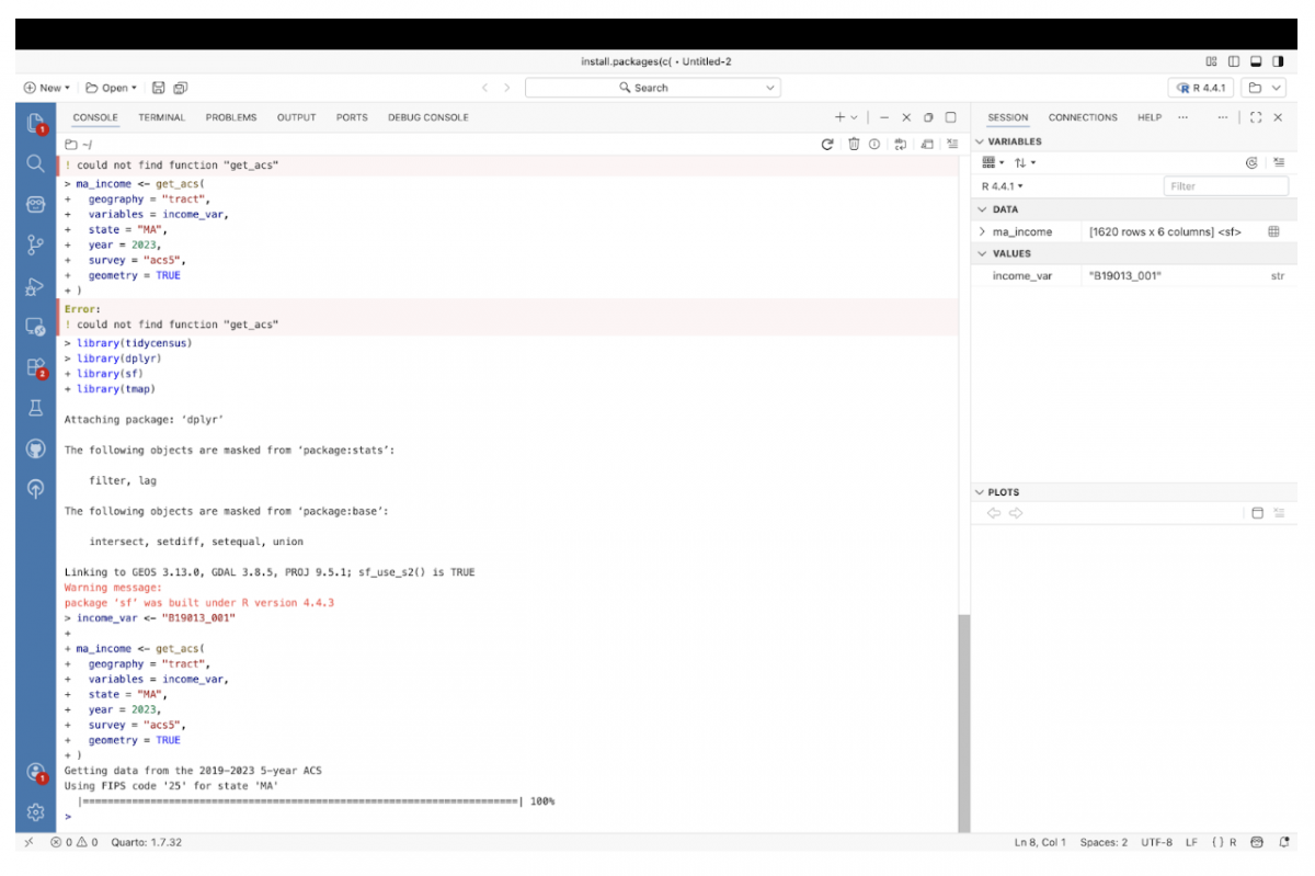

Step 7: Choose a Census variable

For this example, we’ll map median household income, a commonly used ACS variable.

income_var <- "B19013_001"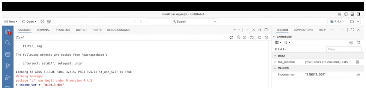

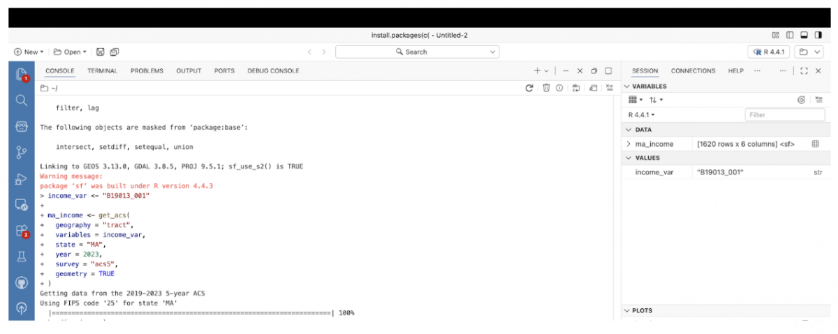
Step 8: Pull Census tract–level ACS data

Use get_acs() to request tract-level data and include geometry in the same call.

ma_income <- get_acs(
geography = "tract",
variables = income_var,
state = "MA",
year = 2023,
survey = "acs5",
geometry = TRUE
)

Setting geometry = TRUE automatically attaches Census tract boundaries, avoiding the need to manually download shapefiles.

If successful, a new object called ma_income will appear in the Variables pane.

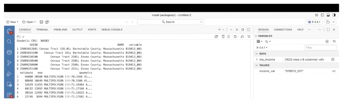
Step 9: Inspect the data

Before mapping, check what the dataset contains.

head(ma_income)

You should see ACS estimates alongside a geometry column, indicating that this is a spatial dataset.

Step 10: Switch tmap to plot mode

Ensure that tmap is set to render static maps.

tmap_mode("plot")

Ignore informational messages about plot versus view modes.

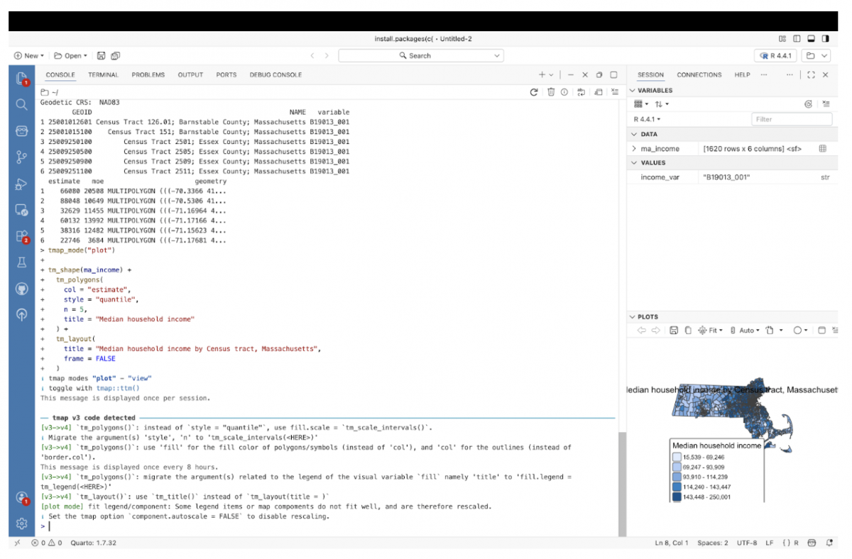
Step 11: Create the Census tract map

Render a basic choropleth map using the ACS estimates.

tm_shape(ma_income) +
  tm_polygons(
    col = "estimate",
    style = "quantile",
    n = 5,
    title = "Median household income"
  ) +
  tm_layout(
    title = "Median household income by Census tract, Massachusetts",
    frame = FALSE
  )

The map will appear in the Plots pane.

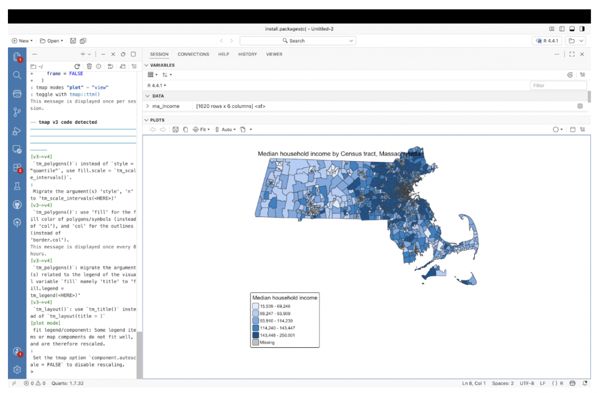
Step 12: View the map at full size

Use the Plots pane’s zoom or pop-out option to view the map in a larger window for readability and screenshots.

Step 13: Export the data as GeoJSON

Save the tract-level dataset for reuse in web maps or other tools.

st_write(ma_income, "ma_income_tracts.geojson", delete_dsn = TRUE)

The file is written to your current working directory.

Step 14: Verify the exported file

Confirm that the file exists.

list.files()

You should see ma_income_tracts.geojson listed. The GeoJSON file can be loaded into any visualization program that does mapping, such as Leaflet, DataWrapper or Flourish.

Why this workflow matters

This approach uses R to pull both census data and tract geometry in one step, avoiding manual downloads and traditional GIS software. For journalism and exploratory analysis, it offers a fast, transparent path from question to map, while keeping the data reusable for future projects.

Census tract data shows up in reporting again and again, from housing and income to language access and public health. Once the data and geography are pulled into R as a single object, the hard part is no longer mapping but deciding what questions to ask next. This workflow is intentionally simple, but it opens the door to deeper analysis, reuse in web projects, or more interactive storytelling. The same steps can be applied to other variables, places, or time periods, making this a flexible starting point rather than a one-off map.