Let’s talk about Python for data analysis. In this tutorial, you will learn some simple data analysis processes while exploring a dataset with Python and Pandas.

Before we get started, make sure you’ve already set up an environment for this practice. Please install Python 3.6, Pandas, and matplotlib. Also, we will use a Jupyter Notebook in this tutorial. If you haven’t heard of the organizational tool, this episode of Linear Digressions does a good job explaining them. 

I will be using Anaconda, a platform for running Python that includes a suite of data analysis tools. This tutorial will be divided into three sections: question, wrangle and explore.

*Download the Jupyter Notebook for this tutorial here.

Decide on your dataset and questions

Data analysis always begins with questions. Those, in turn, will determine what kinds of data you collect. In this tutorial, we are going to explore a dataset of 10,000 news articles collected by NewsWhip between November 2016 and May 2017 posted to Facebook by the top 500 news publishers. We may want to ask which news organizations publish the most articles in the set and what the top keywords are throughout all headlines. 

 

Import the dataset into a Jupyter Notebook

Let’s download our dataset, then import and open it in a Jupyter Notebook. A Jupyter Notebook will start instantly once you type jupyter notebook into Terminal.

 

 

Next, you will get a page like this:

 

 

Next, click the upload button to upload your dataset. Then click the “New” drop-down menu and select Python [conda root].

 

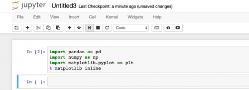
Please follow me to import all the packages we need for this tutorial.

 

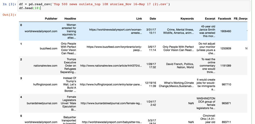
Then, let’s import our dataset by typing

df = pd.read_csv("file_name.csv")

By entering df.head(10), you can review the first 10 rows in this dataset.

 

 

Wrangle

Once we’ve imported the dataset, we need to wrangle the data to help answer the questions we mentioned before. No dataset is perfect and that’s the reason we need to check the issues in this dataset and fix them.

Let’s check how many columns and rows in this dataset by entering df.shape.

 

 

This means we have 10,000 rows and 12 columns. Next, check the data type for each column by entering df.dtypes.

 

 

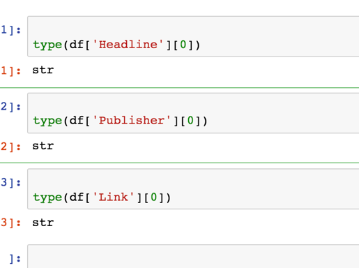
Notice how Publisher, Headline, Link, and Date are all listed as objects. That’s weird. Further investigation shows that they are in fact strings, which I revealed by typing: 

type(df['column name'][0])

 

Converting date column from object into datetime

Let’s change the data type of Date from object to datetime.

Type: df[‘Date’] = pd.to_datetime(df[‘Date’])

After you are done with that, please typing df.dtypes to make sure it works.

 

 

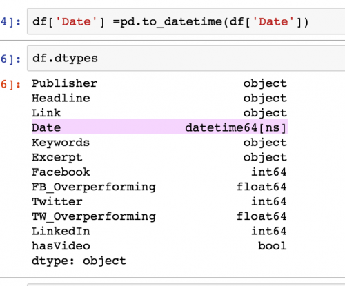
High five! The datatype of Date is now datetime64[ns]. Next, let’s check if we have any missing values in this dataset. We will do so by typing:

df.info()

 

 

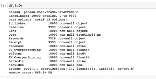
Notice under Keywords that of the 10,000 rows, only 7,528 contain objects in the Keywords column. That means around 2,500 values are missing. That means those articles don’t have keywords. Remember this, because it’s a caveat we’ll need to include when discussing our data analysis.

Next, let’s check if we have any duplicated data by entering df.duplicated()

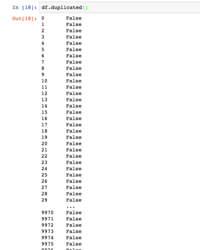
This looks good. We don’t need to drop any duplicated data.

 

Exploring and visualizing the data

Now that you have cleaned your data, you can reveal patterns in our data by using some math operations, such as sum and count. By using the value_counts function, we can count unique values in a column. Then, we can call the plot function on the result to create a bar chart.

Let’s try to count which publisher published the most articles. Type:

 df['column name’].value_counts()

 

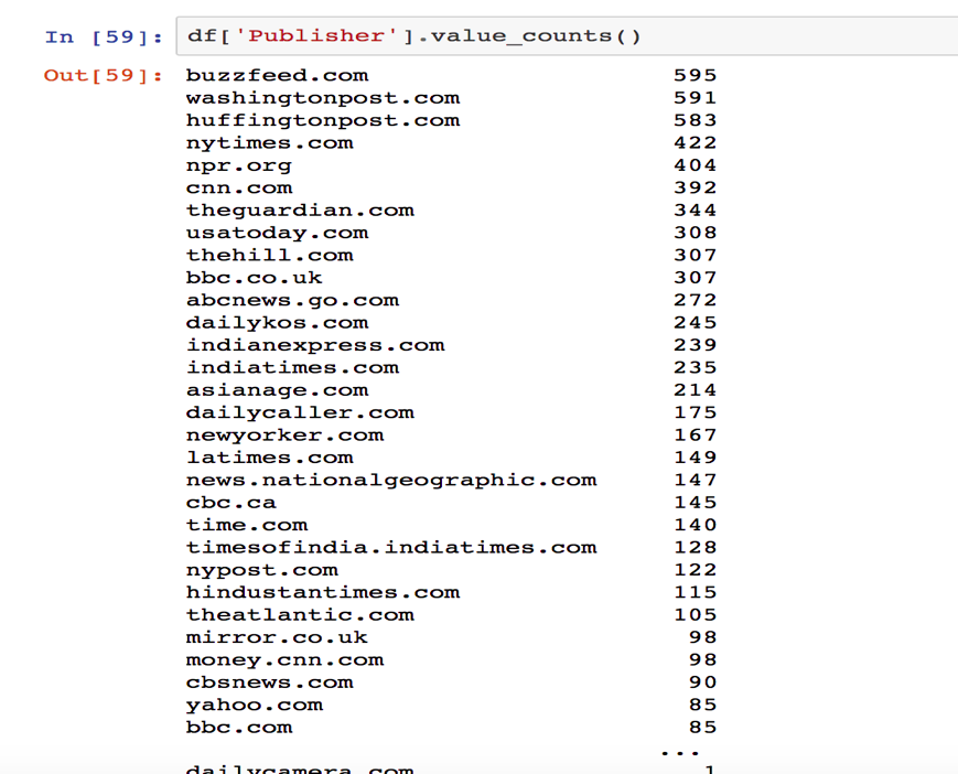
We reveal that BuzzFeed published the most articles in the dataset. To visualize this, we can make a bar chart using matplotlib. One thing that comes in handy when creating visualizations in Jupyter Notebooks is the matplot inline statement, which lets you view your plot in the notebook.

We can use df[‘Publisher’].value_counts().plot(kind = ‘bar’) to draw a simple bar chart. Use figsize to change the size of the plot.

 

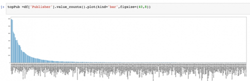
Whoa! This graph is a bit messy. Let’s filter down to the top 10 publishers by descending order.

We can do that by setting up ascending = false, then filter out the top 10 by assigning top10[:10] to the variable top10:

top10 = df["Publisher"].value_counts()
top10.sort_values(ascending=False)
top10 = top10[:10]
top10.plot(kind="bar")

Then, plot that top10 variable by typing: 

top10.plot(kind="bar")

 

 

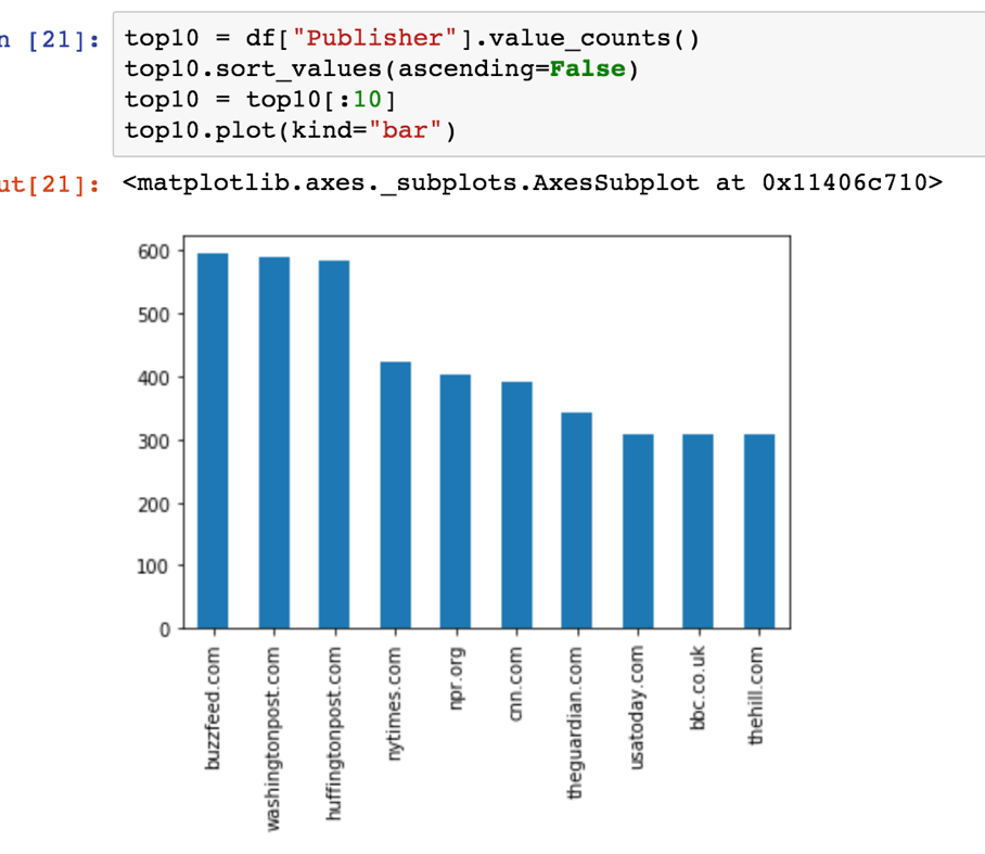
High five! We got our first bar chart!

 

Plotting the top 20 keywords

Next, let’s try to create a bar chart to show the top 20 keywords from the column of Keywords.

This one is little complicated because the keywords are not single words but rather strings of words separated by commas. Without doing that, this is what we visualize:

 

 

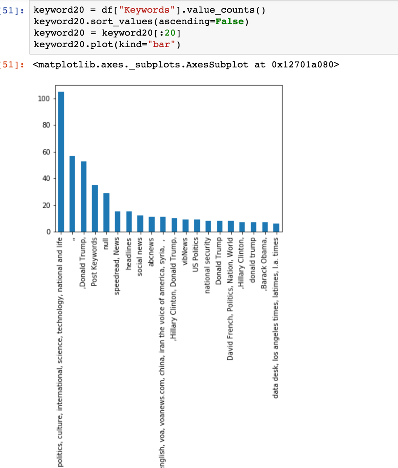
To get an accurate count of the keywords, we need to split the column into single words and put them in arrays – which in Pandas are called series.

Let’s split the column into single words and put them in a series. Then, looping every word in this series, we can get an accurate count of the keywords.

 

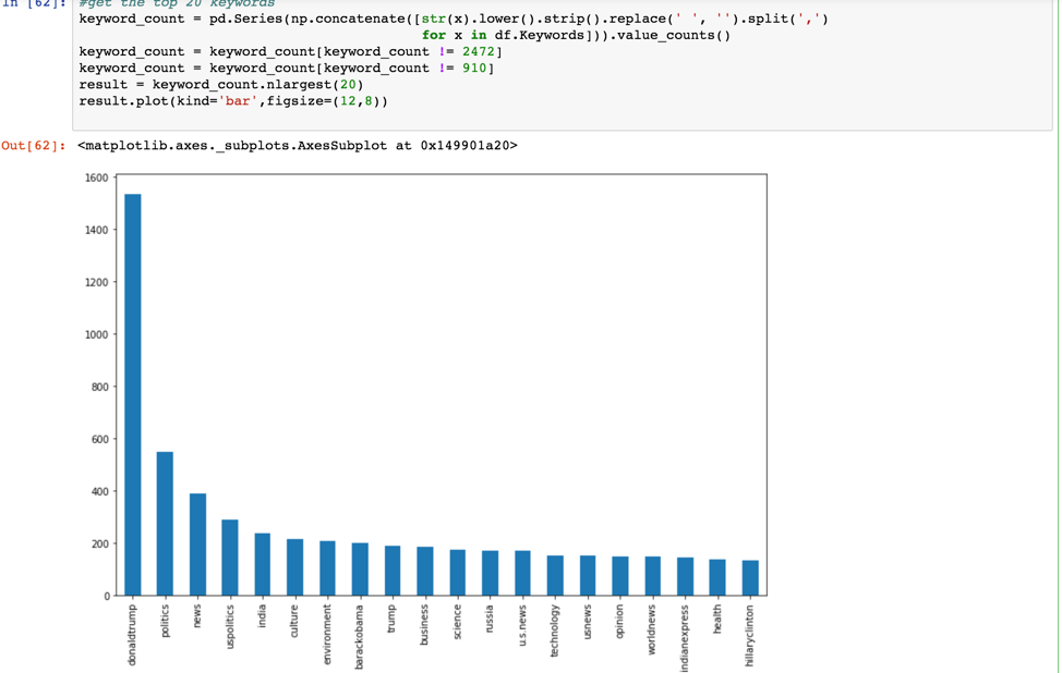
keyword_count = pd.Series(np.concatenate([str(x).lower().strip().replace(' ', '').split(',')
                                          for x in df.Keywords])).value_counts()
keyword_count = keyword_count[keyword_count != 2472]
keyword_count = keyword_count[keyword_count != 910]
result = keyword_count.nlargest(20)
result.plot(kind='bar',figsize=(12,8))
print (keyword_count)

 

Let me explain the code I wrote. The first line is counting the total number of keywords that are Null, then removing them from Series. The second row is counting the total number of keywords which are empty, then removing them from the Series.

We can make a pie chart for this result.

 

 

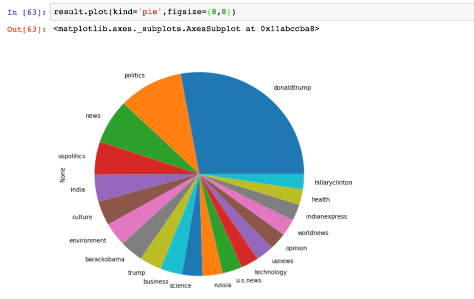
Let’s expand this pie chart for better comparison. It looks so cool!

labels = keyword_count = 'donaldtrump ','politics','news','uspolitics','india','culture','environment','barackobama','russia','u.s.news'
sizes =[1723,549,388,288,236,213,205,199,170,169]
explode =(0.2,0.2,0.2,0.2,0.2,0.2,0.2,0.2,0.3,0.3) 
fig1, ax1 = plt.subplots()
ax1.pie(sizes, explode=explode, labels=labels, autopct='%1.1f%%',
        shadow=True, startangle=90)
ax1.axis('equal')  # Equal aspect ratio ensures that pie is drawn as a circle.

plt.show()

 

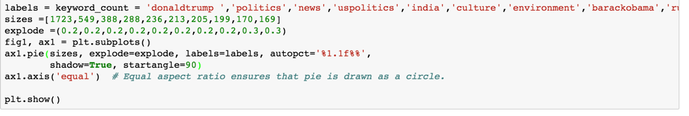
In order to draw this exploded pie chart, we needed to add a few features. Labels are the top 10 keyword we filtered out; Sizes are the total count number of each keyword; Explode splits each label with a different degree – the bigger the number is, the large the gap is; startangle =90 is our custom start angle, which means everything is rotated counter-clockwise by 90 degrees.

*Download the Jupyter Notebook for this tutorial here.

I hope you’ve enjoyed this tutorial. Comments? Suggestions? Get in touch below or at @storybench!