Sentiment analysis is a method of analyzing text data to determine the emotional tone of a message. With the ever-growing volume of text being generated, sentiment analysis provides an opportunity to gain insights into attitudes behind writing on any given topic.

I investigated the disconnect between the benefit of nuclear power as an energy source and the public’s seemingly negative attitudes toward it for my master’s project at Northeastern University School of Journalism’s Media Innovation and Data Communication program. To do so, I conducted a sentiment analysis of The New York Times’ coverage of nuclear energy to see how emotionally-charged language swayed their readers’ opinions of it.

Data collection and cleaning

The first step of any data-driven project is collection. I chose to source articles with the help of Media Cloud. Media Cloud is an open-source tool that generates datasets of articles from major news publishers around the world. It allows users to search news coverage by time period, topic or publisher. Here’s how you can use it to gather the corpus of articles the analysis will be based on.

In this case, we want to search The New York Times for articles related to nuclear energy and nuclear power, across as broad a period of time as possible. We also want to exclude articles about geopolitically fraught issues, such as the Iranian nuclear deal. So we will tell Media Cloud to exclude phrases such as “war,” “bomb” or “missile.”

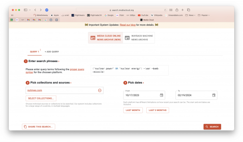
The search should yield six different result categories. We will focus on the sample content.

As shown below, this is a list of 10 observations and three variables: title, source and publication date. Have a look through to ensure the query is fetching content relevant to the search.

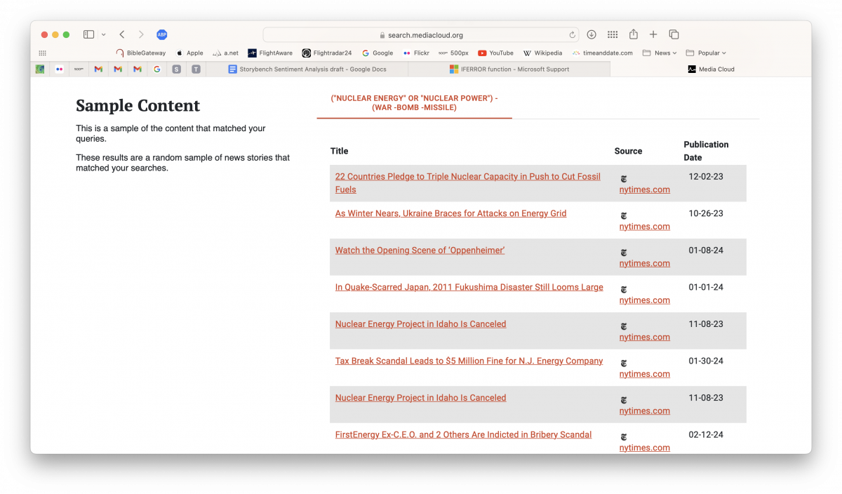
When satisfied, select “Download all URLs,” find the resulting CSV file and open it.

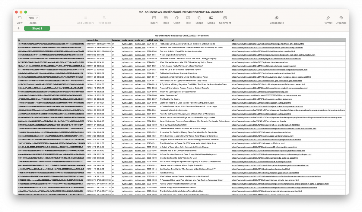
At first glance, the CSV we’ve just downloaded is intimidating. But fear not – most of it is metadata and isn’t important for our purposes. Create a copy of this CSV, then delete every column other than “publish_date,” “title” and “url.” Create a new column to the right, giving it the title of “full_text.”

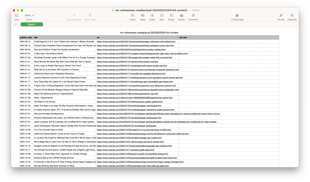
Now, here comes the fun part: manually pulling text from the different webpages. Sure, there probably is a programmatic way of going about this task, but given how few observations there are in the dataset, it is easiest to to fill it in manually.

Another benefit of manually filling in the data is the flexibility it offers. The APIs that Media Cloud relies on are not foolproof. It will occasionally miss content. Being able to manually check for missed content as we fill in the dataset helps to ensure that the data is as comprehensive as possible.

Data processing

Once we have a sufficient amount of data, we can import it into RStudio. But first, we need to load the appropriate packages.

# INSTALL PACKAGES #
install.packages("dplyr")      # Data wrangling
install.packages("ggplot2")    # Visualize data.
install.packages("readr")      # Efficient reading of CSV data.
install.packages("stringr")    # String operations.
install.packages("tibble")     # Convert row names into a column.
install.packages("tidyr")      # Prepare a tidy dataset, gather().
install.packages("tidyverse")  # all tidyverse packages
install.packages("tidytext")   # tidying text data for analysis
install.packages("textdata")   # contains packages useful for text mining
install.packages("ggraph")     # primarily for data visualizations
install.packages("igraph")     # mostly for data structures
install.packages("widyr")      # more data manipulation
install.packages("syuzhet")    # one of many sentiment analysis libraries
install.packages("fmsb")       # to create radar chart
install.packages("reshape2")   # reshape data from wide to long format

# LOAD PACKAGES #
library(dplyr)
library(ggplot2)
library(readr)
library(stringr)
library(tibble)
library(tidyr)
library(tidyverse)
library(tidytext)
library(textdata)
library(ggraph)
library(igraph)
library(widyr)
library(syuzhet)
library(fmsb)
library(reshape2)

Then, load the sentiment models — the libraries that will analyze our text. For this project, we will use the AFINN and NRC lexicon libraries from the tidytext package. The AFINN and NRC lexicons are based on unigrams, or single words.

AFINN assigns a value to each unigram ranging from -5 to 5. Negative numbers correspond with negative sentiment. On the other hand, the NRC lexicon associates each word with one of ten emotions: neutral, fear, negative, positive, trust, sadness, anger, surprise, disgust, joy and anticipation. For the purposes of this project, I included an eleventh category, neutral.

Finally, we need to load the NRC Valence, Arousal and Dominance (NRC VAD) lexicon. The NRC VAD lexicon adds additional dimensions of emotionality that the AFINN or NRC lexicons do not adequately capture.

# LOAD SENTIMENT MODELS #
afinn <- get_sentiments("afinn")
nrc <- get_sentiments("nrc")

# LOAD NRC_VAD LEXICON #
download.file("https://saifmohammad.com/WebDocs/VAD/NRC-VAD-Lexicon-Aug2018Release.zip", destfile="NRCVAD.zip")
unzip("NRCVAD.zip")
Valencedf <- read.table("NRC-VAD-Lexicon-Aug2018Release/OneFilePerDimension/v-scores.txt", header=F, sep="\t")
names(Valencedf) <- c("word","valence")
vdf <- tibble(Valencedf)

Next, we need to load stop words from the “tidytext” package.

“Stop words” are commonly occurring words in a language that, while significant from a grammatical perspective, add little to the semantic meaning of a sentence.

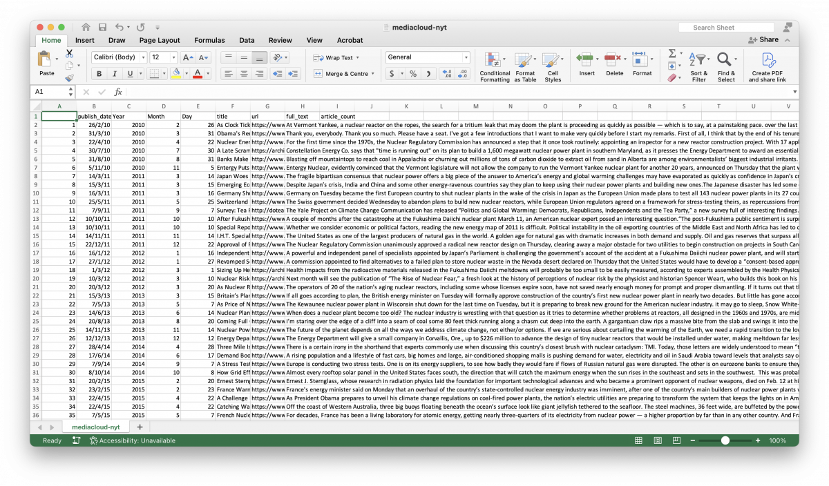
data(stop_words)

Now, we can load our dataset into RStudio.

nyt_10.22 <- read_csv("mediacloud-nyt.csv")

The first thing we want to do is break down the corpus of text data into two-word constructions, or bigrams. Even though the sentiment lexicons in this project are based on monograms, we are trying to find a relationship between emotive language terms related to nuclear energy.

bigrams <- nyt_10.22 %>%
  select(Year, full_text) %>%                                 # selects "Year" and "full_text" variables
  unnest_tokens(bigram, full_text, token="ngrams", n=2) %>%   # splits "full_text" variables into bigrams
  filter(!is.na(bigram)) %>%                                  # removes errors
  separate(bigram, c("word1",
                     "word2"),
           sep=" ") %>%                                       # splits bigrams into two variables
  filter(!word1 %in% stop_words$word,
         !word2 %in% stop_words$word) %>%                     # removes stop words
  filter(word1 == "nuclear") %>%                              # identify bigrams that begin with "nuclear"
  count(Year, word1, word2) %>%
  view()

To assign sentiment categories and values to the bigrams, we need to join the NRC and NRC VAD lexicons to the dataframe we have so far. This is where the lexicon method’s drawbacks start to become apparent. The NRC lexicon library, for instance, is not comprehensive enough to categorize terms related to the technical nature of the nuclear power industry. To this end, we can categorize such terms as “neutral.”

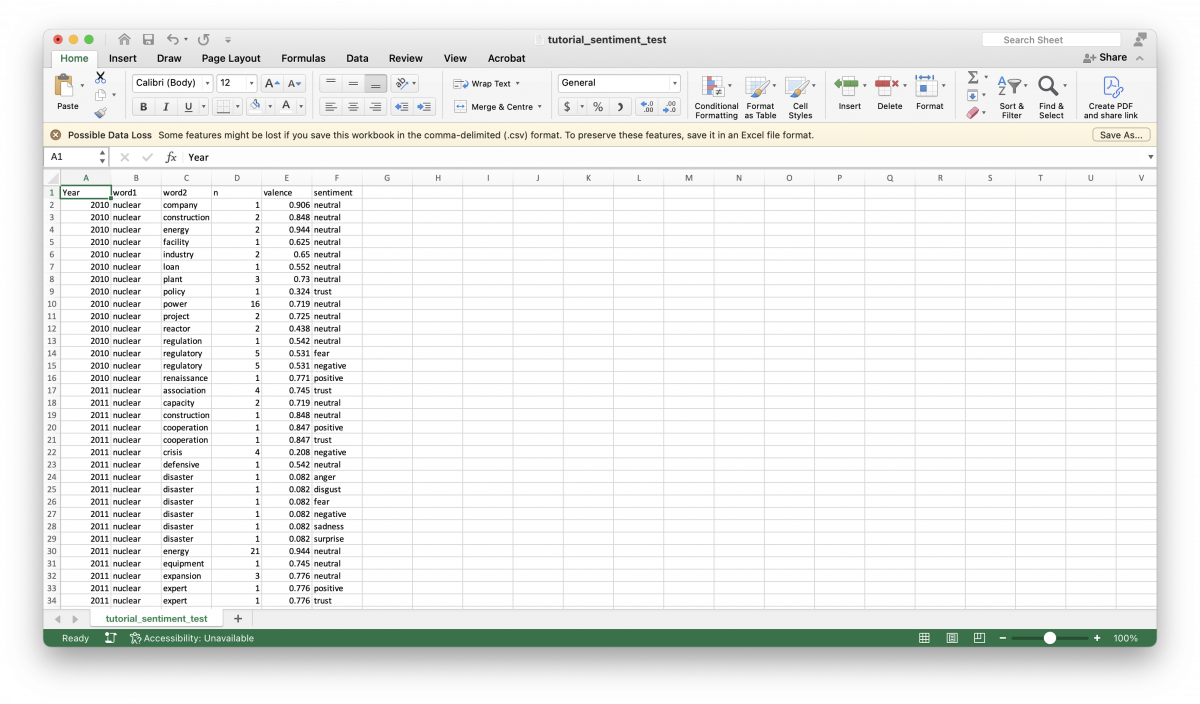
nuclear_bigram_sentiments <- nuclear_bigrams %>%
  left_join(nrc, by = c(word2 = "word")) %>%                # assigns sentiment from NRC lexicon to the second word
  inner_join(vdf, by = c(word2 = "word")) %>%               # assigns sentiment value from NRC_VAD lexicon to the second word
  select(Year, word1, word2, n, sentiment, valence) %>%                # "n" = term frequency; "valence" = sentiment value from NRC VAD lexicon
  view()

nuclear_bigram_sentiments[is.na(nuclear_bigram_sentiments)] <- "neutral"      # replaces "na" values with "neutral"

view(nuclear_bigram_sentiments)

That is how to conduct a sentiment analysis in its simplest form: collect text data, tokenize it and join it to a sentiment lexicon from a text mining package. However, to make it more accessible for a general audience, we need to visualize the data.

Building radar charts

nuclear_bigram_sentiments %>%
  write_csv("[filepath]/bigram_sentiments.csv")

Eagle-eyed readers might have spotted the write_csv() function by now. That is because creating radar charts using the “fmsb” package requires manual data input. For manual input, I prefer to work in Microsoft Excel.

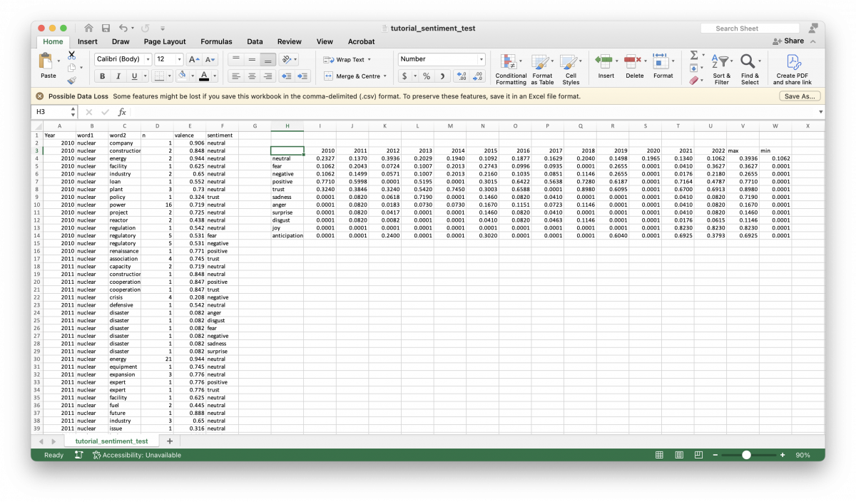
To derive the values needed for the radar chart, we want to work with normalized values. To achieve this, we take the sum of valence values and divide it by the sum of the frequency for each emotional category in a given year.

=IFERROR(SUMIFS($E:$E, $A:$A, I$3, $F:$F, $H4)/SUMIFS($D:$D, $A:$A, I$3, $F:$F, $H4),  0.0001)

Or in plain language, take the sum of valence values, in the year 2010, given a neutral sentiment divided by the sum of a given term’s frequency, in the year 2010, given a neutral sentiment. If the formula returns an error, replace the error with a value of 0.0001. Replacing errors with a value of 0.0001 is important, because the radarchart() function will not properly render charts with a minimum value of 0.

With the normalized, maximum, and minimum values established, we can build the radar charts in RStudio. To do so, we need to build a dataframe using the values we calculated in Excel.

radar_2010 <- data.frame(joy=c(1.215, 0.001, 0.001),
                         surprise=c(12.195, 0.001, 0.001),
                         trust=c(3.086, 0.001, 3.086),
                         positive=c(1.834, 0.001, 1.297),
                         anticipation=c(4.167, 0.001, 0.001),
                         neutral=c(1.731, 1.385, 1.397),
                         anger=c(13.699, 0.001, 0.001),
                         disgust=c(24.390, 0.001, 0.001),
                         fear=c(12.195, 0.001, 1.883),
                         negative=c(18.970, 0.001, 1.883),
                         sadness=c(12.195, 0.001, 0.001))

Note that the data input follows this pattern: c(max_value, min_value, value).

Once we have the dataframe set up, we can call the radarchart() function.

radarchart(radar_2010,
           seg = 10,
           title = "2010",
           # customizing the grid
           cglcol="grey",
           cglty=1,
           axislabcol="grey",
           # customizing the polygon
           pfcol = scales::alpha("green", 0.3), plwd = 2)

For more information about customizing charts, R-Graph-Gallery has fantastic resources.

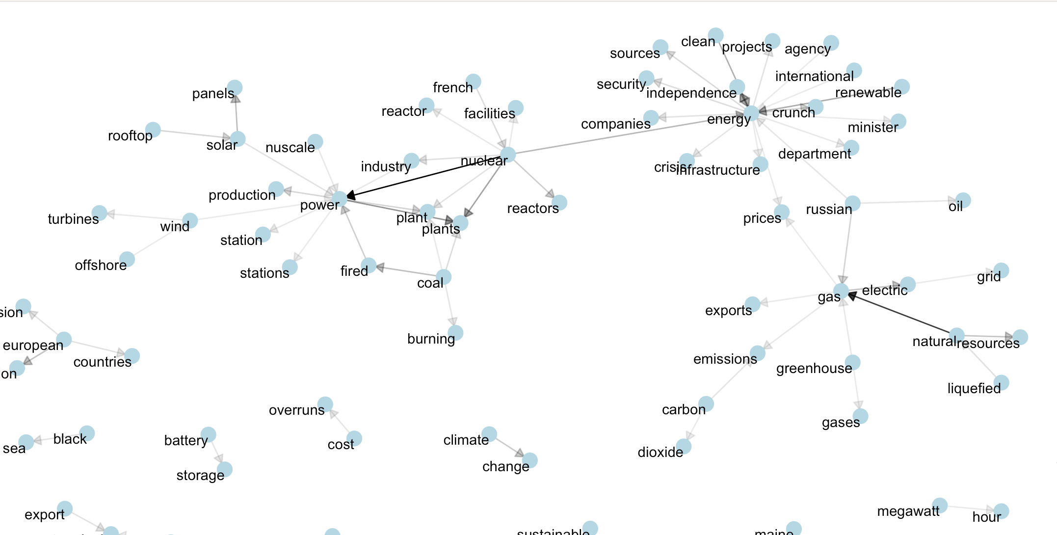
Building network maps

Network maps are a trickier proposition. To help us, we can use the code chunk from the “Text Mining with R” tutorial.

nuclear_bigram_sentiments <- read_csv("[filepath]/nuclear_bigram_sentiments.csv")

set.seed(10)

The set.seed() function generates a set of random values that can be reproduced. We do not need to be overly concerned with this.

filtering_yearly_bigrams <- nuclear_bigram_sentiments %>%
  filter(Year == "2010") %>%
  select(word1, word2, sentiment, n)

bigram_network <- filtering_yearly_bigrams %>%
  filter(n >= 3)

Here, we filter the dataset by year, and the frequency of each bigram’s occurrence. The only factor constraining n is how minimalist or cluttered we want our final network map to appear.

a <- grid::arrow(type = "closed", length = unit(.10, "inches"))

The grid::arrow() function renders an arrow, which for our case, is useful in showing the bigrams that appear in the network maps.

bigram_network %>%
  graph_from_data_frame() %>%
  ggraph(layout = "fr") +
  geom_edge_link(aes(edge_alpha = n),
                 show.legend = FALSE,
                 arrow = a,
                 end_cap = circle(.07, 'inches')) +
  geom_node_point(color = "lightblue", size = 5) +
  geom_node_text(aes(label = name), vjust = 1, hjust = 1) +
  theme_void()

Caveats

This tutorial demonstrates how to execute a sentiment analysis in its simplest form. However, its simplicity means that much of the nuance of language must be sacrificed, thereby rendering the results of a lexicon-based sentiment analysis inconclusive at best.

Sentiment analysis these days benefits from advances in natural language processing (NLP) based on large language models. Huggingface.co is an online platform that hosts models for machine learning tasks. However, it was beyond the scope of this project because knowledge of Python is required.