How to use R to analyze racial profiling at police stops
Working as a data journalist for Eye on Ohio, along with a team of reporters at the Cincinnati Enquirer, I developed a project on the role of racial profiling in police stops in Ohio’s largest cities.
The work was part of Stanford University’s open policing project. Stanford developed the base R script for this — including the “veil of darkness” test, which looks at whether stops are less skewed after dark when police are less likely to see the race of drivers — and gathered some of the records.
A team of Ohio journalists gathered additional records and performed additional analysis. Here’s how we gathered data for Cincinnati (our methodology for all three cities can be seen here.)
First, a few caveats. We compared the population of each city and not the drivers in each city. Because the Ohio Department of Public Safety, which houses the Bureau of Motor Vehicles, does not break down drivers by race, we used data from the United States Census Bureau as a proxy. In addition, our analysis doesn’t account for people driving into and out of the city. Getting a ticket in a city doesn’t necessarily mean you live there.
A note on race: Race is counted two different ways. For a full discussion on this, see The Curious Journalist’s guide to data.
Essentially, “Hispanic” is considered an “ethnicity” and not a “race.” So, you can be white and Hispanic or Black and Hispanic. The actual number of Hispanic people in Cincinnati is quite low, so we went with the definition “non-Hispanic white.” Other caveats:
- We are talking about census blocks here; so the smaller the number counted, the larger the margin of error.
- Geocoding has a block margin of error, since the Cincinnati police code stops as 12XX Main Street. This isn’t a huge error, but it gets larger when we’re talking about a small area like a census block group.
- We had to exclude a small subset of stops that were not properly geocoded or had missing information.
- The “veil of darkness” test assumes that drivers behave the same way at night and during the day. There is some evidence that this is not always the case. See, for example, here. Also, see this Veil of Darkness full paper for a more in-depth analysis. Thank you to the following for providing ggmap: D. Kahle and H. Wickham.
Getting started
First, we need to load the R libraries and data sets for traffic stops in Cincinnati.
## Libraries to include
library(tidyverse)
## ── Attaching packages ──────────────────────────────────────────────────────────────────────────────── tidyverse 1.2.1 ──## ✔ ggplot2 3.2.0 ✔ purrr 0.3.2
## ✔ tibble 2.1.3 ✔ dplyr 0.8.1
## ✔ tidyr 0.8.3 ✔ stringr 1.4.0
## ✔ readr 1.3.1 ✔ forcats 0.4.0## ── Conflicts ─────────────────────────────────────────────────────────────────────────────────── tidyverse_conflicts() ──
## ✖ dplyr::filter() masks stats::filter()
## ✖ dplyr::lag() masks stats::lag()library(lubridate)##
## Attaching package: 'lubridate'## The following object is masked from 'package:base':
##
## datelibrary(dplyr)
library(lutz)
library(suncalc)
library(splines)
library(sf)## Linking to GEOS 3.7.2, GDAL 2.4.2, PROJ 5.2.0library(tabulizer)
library(pdftables)
library(hms)##
## Attaching package: 'hms'## The following object is masked from 'package:lubridate':
##
## hmslibrary(DT)
## Load the data
# Replace the path below with the path to where your data lives on your computer that you are using this script in
#data_path <- "~/Code/SunlightStops/SunlightStopsStory/oh_cincinnati_2019_02_25.csv"
#data_path <- "~/Code/SunlightStops/SunlightStopsStory/CinStopsByBlock2017.csv"
#CINstops <- read_csv(data_path)
#table(CINstops$subject_race)
CINstops <- rio::import("https://stacks.stanford.edu/file/druid:hp256wp2687/hp256wp2687_oh_cincinnati_2019_08_13.csv.zip")
#CINstops <- rio::import("CinStopsWithRaceByBlock.xlsx")
# Additional data and fixed values we'll be using
population_2016 <- tibble(
subject_race = c(
"asian/pacific islander", "black", "hispanic", "other/unknown","white"
),
CINnum_people = c(5418, 127615, 9554, 8489, 145512) #This is where I got this data: https://factfinder.census.gov/faces/tableservices/jsf/pages/productview.xhtml?src=CF
) %>%
mutate(subject_race = as.factor(subject_race))
#Have to add in the latitude and longitude of wherever you are
CINcenter_lat <- 39.1031
CINcenter_lng <- -84.5120This dataset offers most of the information we need, including:
colnames(CINstops)colnames(CINstops)colnames(CINstops)## [1] "raw_row_number" "date"
## [3] "time" "location"
## [5] "lat" "lng"
## [7] "neighborhood" "beat"
## [9] "subject_race" "subject_sex"
## [11] "officer_assignment" "type"
## [13] "disposition" "arrest_made"
## [15] "citation_issued" "warning_issued"
## [17] "outcome" "reason_for_stop"
## [19] "vehicle_make" "vehicle_model"
## [21] "vehicle_registration_state" "vehicle_year"
## [23] "raw_race" "raw_action_taken_cid"
## [25] "raw_field_subject_cid"We can use this command to find out how many stops we have in our dataset:
nrow(CINstops)nrow(CINstops)nrow(CINstops)## [1] 315281summary(CINstops)## raw_row_number date time
## Length:315281 Length:315281 Length:315281
## Class :character Class :character Class :character
## Mode :character Mode :character Mode :character
##
##
##
##
## location lat lng neighborhood
## Length:315281 Min. :-84.69 Min. :-97.60 Length:315281
## Class :character 1st Qu.: 39.11 1st Qu.:-84.54 Class :character
## Mode :character Median : 39.13 Median :-84.52 Mode :character
## Mean : 38.23 Mean :-83.62
## 3rd Qu.: 39.15 3rd Qu.:-84.50
## Max. : 45.53 Max. : 39.27
## NA's :261 NA's :261
## beat subject_race subject_sex
## Length:315281 Length:315281 Length:315281
## Class :character Class :character Class :character
## Mode :character Mode :character Mode :character
##
##
##
##
## officer_assignment type disposition arrest_made
## Length:315281 Length:315281 Length:315281 Mode :logical
## Class :character Class :character Class :character FALSE:269176
## Mode :character Mode :character Mode :character TRUE :45879
## NA's :226
##
##
##
## citation_issued warning_issued outcome reason_for_stop
## Mode :logical Mode :logical Length:315281 Length:315281
## FALSE:132897 FALSE:258896 Class :character Class :character
## TRUE :182158 TRUE :56159 Mode :character Mode :character
## NA's :226 NA's :226
##
##
##
## vehicle_make vehicle_model vehicle_registration_state
## Length:315281 Length:315281 Length:315281
## Class :character Class :character Class :character
## Mode :character Mode :character Mode :character
##
##
##
##
## vehicle_year raw_race raw_action_taken_cid
## Min. : 1932 Length:315281 Length:315281
## 1st Qu.: 1998 Class :character Class :character
## Median : 2002 Mode :character Mode :character
## Mean : 2002
## 3rd Qu.: 2006
## Max. :16998
## NA's :2922
## raw_field_subject_cid
## Length:315281
## Class :character
## Mode :character
##
##
##
## Because the date is a character here, and not a date, we’re changing it to a date format.
CINstops <- filter(CINstops, !is.na(date))
CINstops$date <- as.Date(CINstops$date, format = "%Y-%m-%d")
max(CINstops$date)
## [1] "2018-05-28"Putting times in a time vector:
library(hms)
CINstops$time<-parse_hms(CINstops$time)
Now, we find out the number of stops per year.
CINstops %>%
  group_by(year(date)) %>%
  summarize(Total=n())
## # A tibble: 10 x 2
## `year(date)` Total
## <dbl> <int>
## 1 2009 54630
## 2 2010 52664
## 3 2011 43446
## 4 2012 37876
## 5 2013 25646
## 6 2014 25440
## 7 2015 25372
## 8 2016 21733
## 9 2017 20415
## 10 2018 8059CINstops <- CINstops %>%
filter(year(date) < 2018, year(date) > 2008) #Cincy only has part of 2018 and the data from before 2009 is spotty so we filtered that outWe can sort for only minor stops.
CINstops %>%
  group_by(reason_for_stop) %>%
  summarize(Total=n())
## # A tibble: 146 x 2
## reason_for_stop Total
## <chr> <int>
## 1 <NA> 276001
## 2 --- DISCON CALL 2
## 3 ABDUCTION 1
## 4 ACCIDENT NO INJURIES 53
## 5 ACCIDENT WITH INJURIES 1
## 6 ACCIDENT-VEH INTO BLDG 1
## 7 ADVISED COMPLAINT 22
## 8 ADVISED INCIDENT 9
## 9 ANIMAL COMPLAINT 7
## 10 ASSAULT IN PROGRESS 13
## # … with 136 more rows#unique(CINstops$reason_for_stop)We can also take out anything that doesn’t sound like a traffic stop.
“911 DISCON CALL” “ACCIDENT NO INJURIES” “ACCIDENT WITH INJURIES” “ACCIDENT-VEH INTO BLDG” “ADVISED COMPLAINT”
“ADVISED INCIDENT” “ANIMAL COMPLAINT” “ASSAULT IN PROGRESS” “ASSAULT J/O-NO INJS” “ASSAULT REPORT”
“ATTEMPT TO LOCATE” “AUTO ACC INJ-POL ONL” “AUTO ACCIDENT - NO I” “AUTO ACCIDENT INJURI” “AUTO CRASH INTO BUIL”
, “AUTO THEFT IN PROGRE” “AUTO THEFT J/O” “AUTO THEFT OR RECOVE” “AUTO THEFT REPORT” “B&E REPORT”
,“BACKUP REQUIRED” “BE IN PROG/JO” “BREAKING & ENTERING IN PROGRESS” “CAR IN VIOLATION” “CELL DISCON OR SICAL”
, “CHILD-VICTIM OF CRIM” “COMPLAINT OF PANHAND” “COMPLAINT OF PROSTIT” “CRIMINAL DAMAGING” “CRIMINAL DAMAGING IN”
, “CRIMINAL DAMAGING RE” “CURFEW VIOLATION” “CUTTING IN PROG/JO” “DEFAULT INCIDENT TYP” “DIRECT ALARM”
“DOMESTIC VIOLENCE” “DOMESTIC VIOLENCE J/O” “DRUG ACTIVITY”
, “DRUG COMPLAINT NOT I” “FAMILY TROUBLE” “FAMILY TROUBLE - NON VIOLENT” “FIGHT IN PROGRESS” “FIRE POLICE REQUEST”
, “FIREWORKS” “GENERAL INFO BROADCAST” “GENERAL INFORMATION-” “HEROIN OD” “KEYS LOCKED IN AUTO”
, “LARGE GROUP ASSAULT” “MAINTENANCE RUN” “MEDIA REQUEST FOR IN” “MEET OTHER LAW ENFORCEMENT/AGENCY” “MEET POLICE OFFICER-”
, “MENACING IN PROG/JO” “MENACING J/O” “MENTALLY IMPAIRED NON VIOL” “MENTALLY IMPAIRED VIOL” “MENTALLY IMPAIRED-NO”
, “MISSING PERSON REPOR” “NEIGHBOR TROUBLE” “NEIGHBOR TROUBLE - NON VIOL” “NOISE COMPLAINT” “NON-RESIDENTIAL BURG”
, “NONRESIDENTIAL ALARM DROP” “OFF DUTY POLICE DETAILS” “OFFICER BACKUP/NON ASSISTANCE” “PANHANDLER” “PERS DOWN POL ONLY” “PERSON ARMED W/ GUN” “PERSON ARMED W/WEAPON” “PERSON DOWN - UNK REASON” “PERSON DOWN AND OUT”
, “PERSON W/ WEAPON (OT” “PRISONER” “PROSTITUTE COMPLAINT” “PROWLER” “RAPE J/O OR IN PROGRESS” “REPO” “RESIDENTIAL ALARM DROP” “RESIDENTIAL BURGLAR” “ROBBERY IN PROGRESS-”
, “ROBBERY J/O OR IN PROGRESS” “ROBBERY REPORT” “SERVICE” “SEX OFFENSE OTHER THAN RAPE” “SEX OFFENSES OTHER T”
, “SHOOTING ALREADY OCC” “SHOOTING JO POL ONLY” “SHOT SPOTTER ACTIVITY” “SHOTS FIRED” “SPECIAL DETAIL”
, “STALKING J/O OR IN PROGRESS” “STATION RUN” “STRUCTURE FIRE” “TEST INCIDENT” “THEFT IN PROG/JO” “THEFT J/O OR IN PROGRESS” “THEFT REPORT” “TRANSFERRED CALL” “TRESPASSER” “TRESPASSERS”
,“TOWED VEH - FOR RECORDS USE ONLY” “WARRANT SERVICE”
, “HOLDUP/PANIC ALARM”
We kept these categories:
CINstops <- CINstops %>%
  filter(
    str_detect(reason_for_stop, 'PATROL|DISORD|HAZARD|INV|PARKING|QUERY|SUSPECT|SUSPICIOUS|TRAFFIC|UNKNOWN')| is.na(reason_for_stop))
‘DIRECTED PATROL|DIRECTED PATROL - VEHICLE|DIRECTED PATROL - WALKING|DIRECTED PATROL-WALK| DISORD GROUP|DISORDERLY CROWD|DISORDERLY PERSON|HAZARD TO TRAFFIC/PEDESTRIAN|INV DRUG COMPLAINT|INV POSSIBLE WANTED|INV POSSIBLE WANTED PERSON|INV UNKNOWN TROUBLE|INVESTIGATE|INVESTIGATION|JUVENILE COMPLAINT|PARKING VIOLATION|QUERY|SUSPECT STOP |SUSPICIOUS PERSONS OR SITUATION|SUSPICIOUS SITUATION|TRAFFIC HAZARD|TRAFFIC PURSUIT|TRAFFIC STOP|TRAFFIC TIE|UNKNOWN TROUBLE’), is.na(reason_for_stop))With the categories selected, we could look at arrest rates by race.
ArrestsByRace <- CINstops %>%
  group_by(subject_race, arrest_made) %>%
  summarize(Total =n()) %>%
  group_by(subject_race) %>%
  mutate(pct=Total/sum(Total))
  datatable(ArrestsByRace)
Show 102550100 entries Search:
| subject_race | arrest_made | Total | pct | |
|---|---|---|---|---|
| 1 | asian/pacific islander | false | 1537 | 0.975253807106599 |
| 2 | asian/pacific islander | true | 38 | 0.0241116751269036 |
| 3 | asian/pacific islander | 1 | 0.000634517766497462 | |
| 4 | black | false | 140400 | 0.808751101664161 |
| 5 | black | true | 33081 | 0.190557658078006 |
| 6 | black | 120 | 0.000691240257832616 | |
| 7 | hispanic | false | 419 | 0.843058350100604 |
| 8 | hispanic | true | 78 | 0.156941649899396 |
| 9 | other | false | 20 | 0.952380952380952 |
| 10 | other | true | 1 | 0.0476190476190476 |
Analyzing the data
To begin our analysis, we ran a quick plot of arrests by race.
ArrestsRateByRace <- na.omit(ArrestsByRace)
ggplot(ArrestsRateByRace, aes(x=subject_race, y=Total, fill=arrest_made))+
geom_col(position="dodge")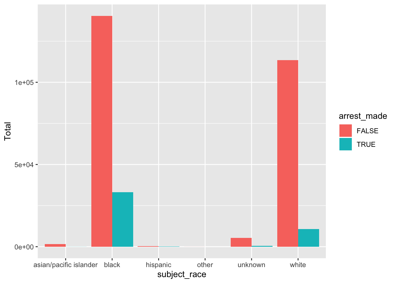
Looking at the arrest percentage overall by race:
Arrest_Percentage_ByRace <- CINstops %>%
  filter(arrest_made=="TRUE") %>%
  group_by(subject_race) %>%
  summarize(Total=n()) %>%
  mutate(pct=Total/sum(Total))
datatable(Arrest_Percentage_ByRace)| subject_race | Total | pct | |
|---|---|---|---|
| 1 | asian/pacific islander | 38 | 0.0008558751323228 |
| 2 | black | 33081 | 0.745084348746593 |
| 3 | hispanic | 78 | 0.00175679632424154 |
| 4 | other | 1 | 0.0000225230297979684 |
| 5 | unknown | 478 | 0.0107660082434289 |
| 6 | white | 10723 | 0.241514448523615 |
We filtered out arrests that were missing latitude/longitude location data.
CINstops <- filter(CINstops, lng!="NA")Filtering to count race:
CINstops %>%
count(subject_race)
## # A tibble: 6 x 2
## subject_race n
## <chr> <int>
## 1 asian/pacific islander 1574
## 2 black 173446
## 3 hispanic 497
## 4 other 21
## 5 unknown 5866
## 6 white 124171
CINstops %>%
count(year = year(date), subject_race) %>%
ggplot(aes(x = year, y = n, color = subject_race)) +
geom_point() +
geom_line()
How stops of particular groups compare to the general population
Here, we are comparing the percentage of traffic stops by race and ethnicity to each group’s percentage of the total population. This creates a proportion:
population_2016 <- population_2016 %>%
mutate(Proportion_Of_Population = CINnum_people / sum(CINnum_people)) #I added this to the populatin data frame
Stops percentage versus population percentage:
StopRateDataTable <- CINstops %>% #I added this table to compare the stop rate versus the population rate
count(subject_race) %>%
left_join(
population_2016,
by = "subject_race"
) %>%
mutate(stop_rate = n / sum(n))
## Warning: Column `subject_race` joining character vector and factor,
## coercing into character vectordatatable(StopRateDataTable)| subject_race | n | CINnum_people | Proportion_Of_Population | stop_rate | |
|---|---|---|---|---|---|
| 1 | asian/pacific islander | 1574 | 5418 | 0.0182677653849785 | 0.00515094493986746 |
| 2 | black | 173446 | 127615 | 0.430277017276491 | 0.567605334206005 |
| 3 | hispanic | 497 | 9554 | 0.0322130362657963 | 0.00162644195369386 |
| 4 | other | 21 | 0.0000687228994518531 | ||
| 5 | unknown | 5866 | 0.0191965965802176 | ||
| 6 | white | 124171 | 145512 | 0.490619984625137 | 0.406351959420764 |
Showing 1 to 6 of 6 entries Previous Next
Calculating the rate of stops (for all cities)
Next, Eye on Ohio calculated the rate of stops for Black people versus white people using a template developed by the Missouri Attorney General. In Cincinnati, at the time, the population was: 49% white, 43% Black and 8% other. Traffic stops were 57% Black, 41% white and 2% other.
We used this formula: the White disparity index value = stop % divided by pop %): (41/49) = 0.8367347
Black DIV: (57/43) = 1.325581
The Black stop rate is 1.58 times that of white stop rate (1.325581/0.8367347).
Thus, accounting for the racial proportion of Cincinnati’s 2016 population, Black people were stopped at a rate 58% higher than white people.
41/49## [1] 0.836734757/43## [1] 1.3255811.325581/0.8367347## [1] 1.584231“Veil of Darkness” test
One way of measuring racial bias is to measure whether the racial imbalance in traffic stops declines after dark when police officers are presumably less able to identify the race of drivers.
Filtering for vehicular data:
CINstops <- CINstops %>% filter(type == "vehicular") #Note this is pretty much all stop dataCINstops <- CINstops %>% filter(type == <span class="hljs-string">"vehicular"</span>) <span class="hljs-comment">#Note this is pretty much all stop data</span>CINstops <- CINstops %>% filter(type == "vehicular") #Note this is pretty much all stop dataCalculating the sunset and dusk times for Cincinnati in 2016:
(Note that we distinguish here between “sunset” and “dusk.” Sunset is the point in time where the sun dips below the horizon. Dusk, also known as the end of civil twilight, is the time when the sun is 6 degrees below the horizon and it is widely considered to be dark. We’ll explain why this is relevant in a moment.)
# Get timezone for Cincinnati
CINtz <- lutz::tz_lookup_coords(CINcenter_lat, CINcenter_lng, warn = F)

# Helper function
time_to_minute <- function(time) {
hour(lubridate::hms(time)) * 60 + minute(lubridate::hms(time))
}

# Compute sunset time for each date in our dataset
sunset_times <-
CINstops %>%
mutate(
lat = CINcenter_lat,
lon = CINcenter_lng
) %>%
select(date, lat, lon) %>%
distinct() %>%
getSunlightTimes(
data = .,
keep = c("dawn","sunrise", "sunset", "dusk"),
tz = CINtz
) %>%
mutate_at(vars("dawn","sunrise","sunset", "dusk"), ~format(., "%H:%M:%S")) %>%
mutate(
  sunset_minute = time_to_minute(sunset),
  dusk_minute = time_to_minute(dusk),
  dawn_minute = time_to_minute(dawn),
  sunrise_minute = time_to_minute(sunrise),
  date = ymd(str_sub(date, 1, 10))
) %>%
  select(date, dawn, sunrise, sunset, dusk, ends_with("minute"))
Great. Now, using sunset_times, what is Cincy’s inter-twilight period?
sunset_times %>%
filter(dusk == min(dusk) | dusk == max(dusk) | dawn == min(dawn) | dawn == max(dawn))
## date dawn sunrise sunset dusk sunset_minute
## 1 2010-06-15 05:40:41 06:12:51 21:06:57 21:39:07 1266
## 2 2017-06-15 05:40:41 06:12:51 21:07:01 21:39:11 1267
## 3 2010-11-06 07:44:28 08:12:29 18:33:30 19:01:30 1113
## 4 2012-06-15 05:40:41 06:12:52 21:07:07 21:39:18 1267
## 5 2016-06-26 05:42:55 06:15:05 21:09:19 21:41:30 1269
## 6 2009-06-14 05:40:41 06:12:50 21:06:40 21:38:49 1266
## 7 2012-12-06 07:15:05 07:44:53 17:16:45 17:46:32 1036
## 8 2016-06-15 05:40:41 06:12:52 21:07:06 21:39:17 1267
## 9 2009-12-06 07:14:54 07:44:41 17:16:45 17:46:32 1036
## 10 2011-06-15 05:40:41 06:12:51 21:06:51 21:39:00 1266
## 11 2010-12-07 07:15:31 07:45:20 17:16:44 17:46:32 1036
## 12 2015-12-07 07:15:16 07:45:04 17:16:44 17:46:32 1036
## 13 2017-06-14 05:40:41 06:12:50 21:06:38 21:38:47 1266
## 14 2011-12-07 07:15:18 07:45:06 17:16:44 17:46:32 1036
## 15 2009-06-15 05:40:41 06:12:52 21:07:02 21:39:13 1267
## 16 2012-06-14 05:40:41 06:12:50 21:06:45 21:38:54 1266
## 17 2010-12-06 07:14:41 07:44:27 17:16:46 17:46:32 1036
## 18 2009-06-27 05:43:14 06:15:23 21:09:20 21:41:30 1269
## 19 2014-12-06 07:14:39 07:44:25 17:16:46 17:46:32 1036
## 20 2016-12-06 07:15:03 07:44:51 17:16:45 17:46:32 1036
## 21 2012-06-26 05:42:55 06:15:06 21:09:19 21:41:30 1269
## 22 2012-06-27 05:43:19 06:15:28 21:09:20 21:41:30 1269
## 23 2017-12-06 07:14:50 07:44:37 17:16:45 17:46:32 1036
## 24 2009-06-26 05:42:51 06:15:01 21:09:19 21:41:30 1269
## 25 2011-12-06 07:14:28 07:44:13 17:16:47 17:46:32 1036
## 26 2010-06-27 05:43:07 06:15:17 21:09:20 21:41:30 1269
## 27 2014-06-15 05:40:41 06:12:51 21:06:56 21:39:06 1266
## 28 2013-06-14 05:40:41 06:12:50 21:06:39 21:38:48 1266
## 29 2015-06-27 05:43:01 06:15:11 21:09:20 21:41:30 1269
## 30 2016-06-14 05:40:41 06:12:50 21:06:44 21:38:53 1266
## 31 2013-06-27 05:43:13 06:15:22 21:09:20 21:41:30 1269
## 32 2017-06-27 05:43:12 06:15:21 21:09:20 21:41:30 1269
## 33 2014-12-07 07:15:29 07:45:18 17:16:44 17:46:32 1036
## 34 2016-06-27 05:43:18 06:15:27 21:09:20 21:41:30 1269
## 35 2013-06-15 05:40:41 06:12:51 21:07:01 21:39:12 1267
## 36 2011-06-27 05:43:01 06:15:12 21:09:20 21:41:30 1269
## 37 2015-06-15 05:40:41 06:12:51 21:06:50 21:39:00 1266
## 38 2014-06-27 05:43:07 06:15:16 21:09:20 21:41:30 1269
## 39 2013-12-06 07:14:52 07:44:39 17:16:45 17:46:32 1036
## dusk_minute dawn_minute sunrise_minute
## 1 1299 340 372
## 2 1299 340 372
## 3 1141 464 492
## 4 1299 340 372
## 5 1301 342 375
## 6 1298 340 372
## 7 1066 435 464
## 8 1299 340 372
## 9 1066 434 464
## 10 1299 340 372
## 11 1066 435 465
## 12 1066 435 465
## 13 1298 340 372
## 14 1066 435 465
## 15 1299 340 372
## 16 1298 340 372
## 17 1066 434 464
## 18 1301 343 375
## 19 1066 434 464
## 20 1066 435 464
## 21 1301 342 375
## 22 1301 343 375
## 23 1066 434 464
## 24 1301 342 375
## 25 1066 434 464
## 26 1301 343 375
## 27 1299 340 372
## 28 1298 340 372
## 29 1301 343 375
## 30 1298 340 372
## 31 1301 343 375
## 32 1301 343 375
## 33 1066 435 465
## 34 1301 343 375
## 35 1299 340 372
## 36 1301 343 375
## 37 1299 340 372
## 38 1301 343 375
## 39 1066 434 464So, we are looking at times between 5:16 p.m. and 9:41 p.m. We need to get those times and take out twilight.
CIN_VODstops <-
CINstops %>%
left_join(
sunset_times,
by = "date"
) %>%
mutate(
minute = time_to_minute(time),
minutes_after_dark = minute - dusk_minute,
is_dark = minute > dusk_minute | minute < dawn_minute,
min_dusk_minute = min(dusk_minute),
max_dusk_minute = max(dusk_minute),
is_black = subject_race == "black"
) %>%
filter(
# Filter to get only the intertwilight period
  ###Skipping this part
#minute >= min_dusk_minute,
minute <= max_dusk_minute,
# Remove ambigous period between sunset and dusk
!(minute > sunset_minute & minute < dusk_minute)
)
Filter to just that time.
CIN_VODstops <- CIN_VODstops %>%
  filter(time > hm("17:16"), time < hm("21:41"))  #Sunset in  winter and summer in Cincy
If you want to only look at highway stops:
CIN_VODstops <- CIN_VODstops %>% filter(str_detect(location, 'I75|I71|I74|I 75|I 71|I 74'))StopsByYearInDarkness <- CIN_VODstops %>%
filter(is_dark) %>%
mutate(year = year(date)) %>%
group_by(year,subject_race) %>%
summarize(Total =n()) %>%
spread(subject_race, Total) %>%
mutate(sunshine = "Darkness")StopsByYearInDaylight <- CIN_VODstops %>%
filter(!is_dark) %>%
mutate(year = year(date)) %>%
group_by(year,subject_race) %>%
summarize(Total =n()) %>%
spread(subject_race, Total)%>%
mutate(sunshine = "Daylight")This adds the two together:
TwilightTable <- rbind(StopsByYearInDarkness, StopsByYearInDaylight) %>%
  group_by(year)
  #View(TwilightTable)
Here are the raw numbers of stops after dark by race:
TwilightTable <- TwilightTable %>%
  mutate(others = `unknown`+`asian/pacific islander`, total_stopped = `black` +`white`+`unknown`+`asian/pacific islander`) %>%
  group_by(year) %>%
  mutate(black_percentage=`black`/total_stopped, white_percentage=white/total_stopped, other_percentage=others/total_stopped)
  datatable(TwilightTable)
TwilightTable <- TwilightTable %>% mutate(others = `unknown`+`asian/pacific islander`, total_stopped = `black` +`white`+`unknown`+`asian/pacific islander`) %>% group_by(year) %>% mutate(black_percentage=`black`/total_stopped, white_percentage=white/total_stopped, other_percentage=others/total_stopped) datatable(TwilightTable)TwilightTable <- TwilightTable %>%
mutate(others = `unknown`+`asian/pacific islander`, total_stopped = `black` +`white`+`unknown`+`asian/pacific islander`) %>%
group_by(year) %>%
mutate(black_percentage=`black`/total_stopped, white_percentage=white/total_stopped, other_percentage=others/total_stopped)
datatable(TwilightTable)| year | asian/pacific islander | black | hispanic | unknown | white | sunshine | others | total_stopped | black_percentage | white_percentage | other_percentage | |
|---|---|---|---|---|---|---|---|---|---|---|---|---|
| 1 | 2009 | 13 | 170 | 4 | 13 | 520 | Darkness | 26 | 716 | 0.237430167597765 | 0.726256983240223 | 0.0363128491620112 |
| 2 | 2010 | 9 | 145 | 5 | 16 | 485 | Darkness | 25 | 655 | 0.221374045801527 | 0.740458015267176 | 0.0381679389312977 |
| 3 | 2011 | 10 | 118 | 8 | 349 | Darkness | 18 | 485 | 0.243298969072165 | 0.719587628865979 | 0.0371134020618557 | |
| 4 | 2012 | 3 | 95 | 13 | 309 | Darkness | 16 | 420 | 0.226190476190476 | 0.735714285714286 | 0.0380952380952381 | |
| 5 | 2013 | 6 | 145 | 18 | 327 | Darkness | 24 | 496 | 0.292338709677419 | 0.659274193548387 | 0.0483870967741935 | |
| 6 | 2014 | 8 | 100 | 15 | 238 | Darkness | 23 | 361 | 0.277008310249307 | 0.659279778393352 | 0.0637119113573407 | |
| 7 | 2015 | 4 | 88 | 13 | 222 | Darkness | 17 | 327 | 0.269113149847095 | 0.678899082568807 | 0.0519877675840979 | |
| 8 | 2016 | 2 | 79 | 13 | 128 | Darkness | 15 | 222 | 0.355855855855856 | 0.576576576576577 | 0.0675675675675676 | |
| 9 | 2017 | 1 | 59 | 7 | 121 | Darkness | 8 | 188 | 0.313829787234043 | 0.643617021276596 | 0.0425531914893617 | |
| 10 | 2009 | 15 | 198 | 8 | 20 | 705 | Daylight | 35 | 938 | 0.211087420042644 | 0.751599147121535 | 0.0373134328358209 |
This looks at the percentage of Black people and percentage of white people stopped in daylight, and during the same time period but because of the time change, in darkness:
TwilightTable <- TwilightTable %>%
  mutate(others = `unknown`+`asian/pacific islander`, total_stopped = `black` +`white`+`unknown`+`asian/pacific islander`) %>%
  group_by(year) %>%
  mutate(black_percentage=`black`/total_stopped, white_percentage=white/total_stopped, other_percentage=others/total_stopped)
datatable(TwilightTable)| year | asian/pacific islander | black | hispanic | unknown | white | sunshine | others | total_stopped | black_percentage | white_percentage | other_percentage | |
|---|---|---|---|---|---|---|---|---|---|---|---|---|
| 1 | 2009 | 13 | 170 | 4 | 13 | 520 | Darkness | 26 | 716 | 0.237430167597765 | 0.726256983240223 | 0.0363128491620112 |
| 2 | 2010 | 9 | 145 | 5 | 16 | 485 | Darkness | 25 | 655 | 0.221374045801527 | 0.740458015267176 | 0.0381679389312977 |
| 3 | 2011 | 10 | 118 | 8 | 349 | Darkness | 18 | 485 | 0.243298969072165 | 0.719587628865979 | 0.0371134020618557 | |
| 4 | 2012 | 3 | 95 | 13 | 309 | Darkness | 16 | 420 | 0.226190476190476 | 0.735714285714286 | 0.0380952380952381 | |
| 5 | 2013 | 6 | 145 | 18 | 327 | Darkness | 24 | 496 | 0.292338709677419 | 0.659274193548387 | 0.0483870967741935 | |
| 6 | 2014 | 8 | 100 | 15 | 238 | Darkness | 23 | 361 | 0.277008310249307 | 0.659279778393352 | 0.0637119113573407 | |
| 7 | 2015 | 4 | 88 | 13 | 222 | Darkness | 17 | 327 | 0.269113149847095 | 0.678899082568807 | 0.0519877675840979 | |
| 8 | 2016 | 2 | 79 | 13 | 128 | Darkness | 15 | 222 | 0.355855855855856 | 0.576576576576577 | 0.0675675675675676 | |
| 9 | 2017 | 1 | 59 | 7 | 121 | Darkness | 8 | 188 | 0.313829787234043 | 0.643617021276596 | 0.0425531914893617 | |
| 10 | 2009 | 15 | 198 | 8 | 20 | 705 | Daylight | 35 | 938 | 0.211087420042644 | 0.751599147121535 | 0.0373134328358209 |
Showing 1 to 10 of 18 entries
This looks at the percentage of Black people and the percentage of white people stopped in daylight, and during the same time period but because of the time change, in darkness:
TwilightTableTogether <- TwilightTable %>%
  group_by(sunshine) %>%
  summarize(Percent_Of_Blacks_Stopped=mean(black_percentage),
         Percent_of_Whites_Stopped=mean(white_percentage),
         other=mean(other_percentage))
  datatable(TwilightTableTogether)
Show 102550100 entriesSearch:
| sunshine | Percent_Of_Blacks_Stopped | Percent_of_Whites_Stopped | other | |
|---|---|---|---|---|
| 1 | Darkness | 0.270715496836184 | 0.682184840605709 | 0.0470996625581071 |
| 2 | Daylight | 0.276210083612077 | 0.671518460364006 | 0.052271456023917 |
Now, the same analysis, but with non-highway vehicular stops. (If you’re stopping someone on foot, you can see that person in daylight or darkness.) We’re bringing in Cincinnati stops again and getting the data to the format we want.
CINstops <- rio::import("https://stacks.stanford.edu/file/druid:hp256wp2687/hp256wp2687_oh_cincinnati_2019_08_13.csv.zip")

CINstops <- filter(CINstops, !is.na(date))
CINstops$date <- as.Date(CINstops$date, format = "%Y-%m-%d")

CINstops <- CINstops %>%
  filter(year(date) < 2017, year(date) > 2008) %>%
  filter(type == "vehicular")

CINstops$time<-parse_hms(CINstops$time)

CINstops <- CINstops %>%
  filter(
    str_detect(reason_for_stop, 'PATROL|DISORD|HAZARD|INV|PARKING|QUERY|SUSPECT|SUSPICIOUS|TRAFFIC|UNKNOWN')| is.na(reason_for_stop))
CIN_VODstops <-
CINstops %>%
left_join(
sunset_times,
by = "date"
) %>%
mutate(
minute = time_to_minute(time),
minutes_after_dark = minute - dusk_minute,
is_dark = minute > dusk_minute | minute < dawn_minute,
min_dusk_minute = min(dusk_minute),
max_dusk_minute = max(dusk_minute),
is_black = subject_race == "black"
) %>%
filter(
# Filter to get only the intertwilight period
###Skipping this part
#minute >= min_dusk_minute,
minute <= max_dusk_minute,
# Remove ambigous period between sunset and dusk
!(minute > sunset_minute & minute < dusk_minute)
)Filter to just that time.
CIN_VODstops <- CIN_VODstops %>%
  filter(time > hm("17:16"), time < hm("21:41"))  #Sunset in  winter and summer in Cincy
If you want to only look at street stops:
CIN_VODstops <- CIN_VODstops %>% filter(!str_detect(location, 'I75|I71|I74|I 75|I 71|I 74'))StopsByYearInDarkness <- CIN_VODstops %>%
filter(is_dark) %>%
mutate(year = year(date)) %>%
group_by(year,subject_race) %>%
summarize(Total =n()) %>%
spread(subject_race, Total) %>%
mutate(sunshine = "Darkness")StopsByYearInDaylight <- CIN_VODstops %>%
filter(!is_dark) %>%
mutate(year = year(date)) %>%
group_by(year,subject_race) %>%
summarize(Total =n()) %>%
spread(subject_race, Total)%>%
mutate(sunshine = "Daylight")This creates a “twilight table” which puts into one spreadsheet all the vehicular stops per year that occur at the same time, but because of the time change will be in either daylight or darkness.
Here are the raw numbers:
TwilightTable <- TwilightTable %>%
  mutate(other = `unknown`+`asian/pacific islander`, total_stopped = `black` +`white`+`unknown`+`asian/pacific islander`) %>%
  group_by(year) %>%
  mutate(black_percentage=`black`/total_stopped, white_percentage=white/total_stopped, other_percentage=other/total_stopped)
  datatable(TwilightTable)
Show 102550100 entriesSearch:
| year | asian/pacific islander | black | hispanic | other | unknown | white | sunshine | total_stopped | black_percentage | white_percentage | other_percentage | |
|---|---|---|---|---|---|---|---|---|---|---|---|---|
| 1 | 2009 | 23 | 3441 | 8 | 90 | 67 | 1790 | Darkness | 5321 | 0.646682954331892 | 0.336402931779741 | 0.0169141138883668 |
| 2 | 2010 | 19 | 3224 | 9 | 89 | 70 | 1440 | Darkness | 4753 | 0.678308436776773 | 0.30296654744372 | 0.0187250157795077 |
| 3 | 2011 | 19 | 2071 | 89 | 70 | 1044 | Darkness | 3204 | 0.646379525593009 | 0.325842696629214 | 0.0277777777777778 | |
| 4 | 2012 | 22 | 1798 | 76 | 54 | 946 | Darkness | 2820 | 0.637588652482269 | 0.335460992907801 | 0.0269503546099291 | |
| 5 | 2013 | 8 | 1034 | 39 | 31 | 609 | Darkness | 1682 | 0.61474435196195 | 0.362068965517241 | 0.0231866825208086 | |
| 6 | 2014 | 4 | 1119 | 31 | 27 | 507 | Darkness | 1657 | 0.675316837658419 | 0.305974652987327 | 0.0187085093542547 | |
| 7 | 2015 | 11 | 1381 | 42 | 31 | 686 | Darkness | 2109 | 0.654812707444286 | 0.325272641062115 | 0.0199146514935989 | |
| 8 | 2016 | 7 | 1081 | 44 | 37 | 606 | Darkness | 1731 | 0.624494511842865 | 0.350086655112652 | 0.025418833044483 | |
| 9 | 2009 | 18 | 3543 | 30 | 88 | 70 | 1805 | Daylight | 5436 | 0.651766004415011 | 0.332045621780721 | 0.0161883738042678 |
| 10 | 2010 | 21 | 3762 | 20 | 72 | 51 | 1836 | Daylight | 5670 | 0.663492063492063 | 0.323809523809524 | 0.0126984126984127 |
Showing 1 to 10 of 16 entries
This looks at the percentage of Black people and the percentage of white people stopped in daylight, and during the same time period but because of the time change, in darkness.
TwilightTableTogether <- TwilightTable %>%
  group_by(sunshine) %>%
  summarize(Percent_Of_Blacks_Stopped=mean(black_percentage),
         Percent_of_Whites_Stopped=mean(white_percentage),
         other=mean(other_percentage))
datatable(TwilightTableTogether)| sunshine | Percent_Of_Blacks_Stopped | Percent_of_Whites_Stopped | other | |
|---|---|---|---|---|
| 1 | Darkness | 0.647290997261433 | 0.330509510429976 | 0.0221994923085908 |
| 2 | Daylight | 0.646946366491183 | 0.334666246487957 | 0.0183873870208602 |
Showing 1 to 2 of 2 entries
Finally, let’s map what we’ve found
We plot the stops by neighborhood to provide more detail. Start by downloading data from CensusReporter.org where we can find the shape files. Next, we get race info for each neighborhood from the census.
#You'll have to set your file pane location here
CincyRaceInfoByLocation2 <- sf::st_read("acs2017_5yr_B02001_15000US390610047011.shp") %>%
mutate(
  Total=B02001001,
  White_Alone=B02001002,
  Black_Alone=B02001003,
  PctWhite = round((White_Alone/Total)*100, 1),
  PctBlack = round((Black_Alone/Total)*100, 1)) %>%
slice(-n())
## Reading layer `acs2017_5yr_B02001_15000US390610047011' from data source `/Users/Lucia/Code/SunlightStops/SunlightStopsStory/acs2017_5yr_B02001_15000US390610047011.shp' using driver `ESRI Shapefile'
## Simple feature collection with 298 features and 22 fields
## geometry type: POLYGON
## dimension: XY
## bbox: xmin: -84.71216 ymin: 39.05188 xmax: -84.3454 ymax: 39.22502
## epsg (SRID): 4326
## proj4string: +proj=longlat +datum=WGS84 +no_defsNow, we’re taking a look at our Cincinnati neighborhood stops.
# We only need the columns with the latitude and longitude

CINstops <- rio::import("https://stacks.stanford.edu/file/druid:hp256wp2687/hp256wp2687_oh_cincinnati_2019_08_13.csv.zip")

CINstops <- filter(CINstops, !is.na(date))
CINstops$date <- as.Date(CINstops$date, format = "%Y-%m-%d")

CINstops <- CINstops %>%
  filter(year(date) < 2017, year(date) > 2008)

CINstops$time<-parse_hms(CINstops$time)

# Check and eliminate the rows that don't have location information
CINstops <- CINstops %>%
  filter(lat!="NA")

CINstops <- CINstops %>%
  filter(
    str_detect(reason_for_stop, 'PATROL|DISORD|HAZARD|INV|PARKING|QUERY|SUSPECT|SUSPICIOUS|TRAFFIC|UNKNOWN')| is.na(reason_for_stop))
Filter to only neighborhoods and take out Antarctica. (A small number may have gotten their latitude and longitude mixed up, which gave us points in Antarctica.)
#We need the street stops only here. Stopping somone on the highway is not really "in" a neighborhood

CINstops <- CINstops %>%
  filter(!lat<1,!lng>1) %>%
  filter(!str_detect(location,'I75|I71|I74|I 75|I 71|I 74'))
  #filter(type=="vehicular", lat<46, lng>1)
Now, we can summarize the data by count and merge it back to the shape file and visualize it.
#Or, Getting Hamilton block groups (Cincinnati is entirely within Hamilton County)
library(tigris)
## To enable
## caching of data, set `options(tigris_use_cache = TRUE)` in your R script or .Rprofile.##
## Attaching package: 'tigris'## The following object is masked from 'package:graphics':
##
## plotoptions(tigris_class = "sf")
HamiltonBlockGroups <- block_groups("OH",county = "Hamilton")
CINstops_spatial <- CINstops %>%
st_as_sf(coords=c("lng", "lat"), crs="+proj=longlat") %>%
st_transform(crs=st_crs(HamiltonBlockGroups))
#Putting them altogether
CINStopsWithTracts <- st_join(HamiltonBlockGroups, CINstops_spatial)## although coordinates are longitude/latitude, st_intersects assumes that they are planar#Vlookup
CINStopsWithTracts$GEOID <- paste0("15000US",CINStopsWithTracts$GEOID)This puts the stops and race percentage of each block together.
CINstops_With_Race_and_Tracts <-  CINStopsWithTracts

CINstops_With_Race_and_Tracts$PctWhite = CincyRaceInfoByLocation2$PctWhite[match(CINStopsWithTracts$GEOID, CincyRaceInfoByLocation2$geoid)]


CINstops_With_Race_and_Tracts$PctBlack = CincyRaceInfoByLocation2$PctBlack[match(CINStopsWithTracts$GEOID, CincyRaceInfoByLocation2$geoid)]

CINstops_With_Race_and_Tracts$Total_People_Per_Census_Block = CincyRaceInfoByLocation2$Total[match(CINStopsWithTracts$GEOID, CincyRaceInfoByLocation2$geoid)]
Finding the total number of stops per resident in neighborhoods with at least 0.7% white or Black residents:
CINstops_With_Race_and_Tracts <- CINstops_With_Race_and_Tracts %>%
  filter(PctWhite!="NA", PctBlack!="NA")

Mostly_White_Cincy <- CINstops_With_Race_and_Tracts %>%
filter(PctWhite>75) %>%
group_by(GEOID) %>%
summarize(
Total=n(), Per_Capita=Total/mean(Total_People_Per_Census_Block), Total_In_Block=mean(Total_People_Per_Census_Block))


Mostly_Black_Cincy <- CINstops_With_Race_and_Tracts %>%
filter(PctBlack>75) %>%
group_by(GEOID) %>%
summarize(
Total=n(), Per_Capita=Total/mean(Total_People_Per_Census_Block), Total_In_Block=mean(Total_People_Per_Census_Block))


Mixed_Cincy <- CINstops_With_Race_and_Tracts %>%
filter(!PctBlack>75|!PctWhite>75) %>%
group_by(GEOID) %>%
summarize(
Total=n(), Per_Capita=Total/mean(Total_People_Per_Census_Block), Total_In_Block=mean(Total_People_Per_Census_Block))


mean(Mostly_White_Cincy$Per_Capita)
## [1] 0.5271393mean(Mostly_Black_Cincy$Per_Capita)## [1] 1.311483This looks at the rate in all predominantly Black areas and all predominantly white areas together and calculates how much more likely stops were in predominantly Black areas:
Total_People_In_Mostly_White_Cincy_Blocks <- sum(Mostly_White_Cincy$Total_In_Block)
Total_People_In_Mostly_Black_Cincy_Blocks <- sum(Mostly_Black_Cincy$Total_In_Block)
Total_People_In_Mixed_Blocks <-sum(Mixed_Cincy$Total_In_Block)

Total_Stops_In_Mostly_White_Cincy_Blocks <-sum(Mostly_White_Cincy$Total)
Total_Stops_In_Mostly_Black_Cincy_Blocks <-sum(Mostly_Black_Cincy$Total)
Total_Stops_In_Mixed_Blocks <-sum(Mixed_Cincy$Total)


Total_Stops_In_Mostly_White_Cincy_Blocks/Total_People_In_Mostly_White_Cincy_Blocks
## [1] 0.3992041Total_Stops_In_Mostly_Black_Cincy_Blocks/Total_People_In_Mostly_Black_Cincy_Blocks## [1] 0.8788373CIN_white_rate <- Total_Stops_In_Mostly_White_Cincy_Blocks/Total_People_In_Mostly_White_Cincy_Blocks
CIN_black_rate <- Total_Stops_In_Mostly_Black_Cincy_Blocks/Total_People_In_Mostly_Black_Cincy_Blocks
(CIN_black_rate-CIN_white_rate)/CIN_white_rate## [1] 1.201474The published investigation prompted outrage in the Black community, particularly in Cincinnati where it was a hot topic at city hall meetings. The chief of police there defended the disparities we showed saying that putting officers in high crime areas helped to decrease response times. In contrast, Cincinnati Councilman Jeff Pastor called for a review of racial disparities in traffic stops in December of 2019. Of course a few months later the issue became even more heated following the death of George Floyd and subsequent protests. The city hall later added more funds to the Citizen Complaint Authority, which critics argued had been underfunded for years.

- How to Analyze bluesky Posts and Trends with R - November 4, 2025
- Easily clean up messy databases with fuzzy matching in R - September 16, 2025
- How to use R to analyze racial profiling at police stops - November 21, 2023