How to model with gradient boosting machine in R
The tutorial is part 2 of our #tidytuesday post from last week, which explored bike rental data from Washington, D.C. Check it out here. The following tutorial will use a gradient boosting machine (GBM) to figure out what drives bike rental behavior.
GBM is unique compared to other decision tree algorithms because it builds models sequentially with higher weights given to those cases that were poorly predicted in previous models, thus improving accuracy incrementally instead of simply taking an average of all models like a random forest algorithm would. By reducing the error iteratively to produce what will become the final model, GBM is an efficient and powerful algorithm for classification and regression problems.
Implementing GBM in R allows for a nice selection of exploratory plots including parameter contribution, and partial dependence plots which provide a visual representation of the effect across values of a feature in the model.
Load the packages
The packages below are needed to complete this analysis.
# packages --------------------------------------------------------------
library(rsample)
library(caret)
library(ggthemes)
library(scales)
library(wesanderson)
library(tidyverse)
library(gbm)
library(Metrics)
library(here)
Run previous scripts to import and wrangle data.
base::source("code/01-import.R")
base::source("code/02.3-wrangle.R")
base::source("code/03.3-visualize.R") # we don't neeed to run 03-vizualize.R,
# because it does not change the underlying data structure, but we wantto view
# the EDA outputs
What did we learn in part 1?
The exploratory data analysis showed us that bike rentals seem to drop off at a certain temperature (~20˚C).
ggRentalsByTemp
And that rentals were lower on holidays compared to non-holidays.

So now that we have some understanding of the variables in BikeData, we can use the Generalized Boosted Regression Models (gbm) package to model the bike rental data.
The data
BikeData %>% glimpse()
    ## Observations: 731
    ## Variables: 30
    ## $ weekday         6, 0, 1, 2, 3, 4, 5, 6, 0, 1, 2, 3, 4, 5, 6, 0, 1, 2…
    ## $ weekday_chr     "Saturday", "Sunday", "Monday", "Tuesday", "Wednesda…
    ## $ weekday_fct     Saturday, Sunday, Monday, Tuesday, Wednesday, Thursd…
    ## $ holiday         0, 0, 0, 0, 0, 0, 0, 0, 0, 0, 0, 0, 0, 0, 0, 0, 1, 0…
    ## $ holiday_chr     "Non-Holiday", "Non-Holiday", "Non-Holiday", "Non-Ho…
    ## $ holiday_fct     Non-Holiday, Non-Holiday, Non-Holiday, Non-Holiday, …
    ## $ season          1, 1, 1, 1, 1, 1, 1, 1, 1, 1, 1, 1, 1, 1, 1, 1, 1, 1…
    ## $ season_chr      "Spring", "Spring", "Spring", "Spring", "Spring", "S…
    ## $ season_fct      Spring, Spring, Spring, Spring, Spring, Spring, Spri…
    ## $ workingday      0, 0, 1, 1, 1, 1, 1, 0, 0, 1, 1, 1, 1, 1, 0, 0, 0, 1…
    ## $ workingday_chr  "Non-Working Day", "Non-Working Day", "Working Day",…
    ## $ workingday_fct  Non-Working Day, Non-Working Day, Working Day, Worki…
    ## $ month_ord       Jan, Jan, Jan, Jan, Jan, Jan, Jan, Jan, Jan, Jan, Ja…
    ## $ month_fct       January, January, January, January, January, January…
    ## $ yr              0, 0, 0, 0, 0, 0, 0, 0, 0, 0, 0, 0, 0, 0, 0, 0, 0, 0…
    ## $ yr_chr          "2011", "2011", "2011", "2011", "2011", "2011", "201…
    ## $ yr_fct          2011, 2011, 2011, 2011, 2011, 2011, 2011, 2011, 2011…
    ## $ weathersit      2, 2, 1, 1, 1, 1, 2, 2, 1, 1, 2, 1, 1, 1, 2, 1, 2, 2…
    ## $ weathersit_chr  "Clouds/Mist", "Clouds/Mist", "Good", "Good", "Good"…
    ## $ weathersit_fct  Clouds/Mist, Clouds/Mist, Good, Good, Good, Good, Cl…
    ## $ instant         1, 2, 3, 4, 5, 6, 7, 8, 9, 10, 11, 12, 13, 14, 15, 1…
    ## $ dteday          2011-01-01, 2011-01-02, 2011-01-03, 2011-01-04, 201…
    ## $ mnth            1, 1, 1, 1, 1, 1, 1, 1, 1, 1, 1, 1, 1, 1, 1, 1, 1, 1…
    ## $ temp            8, 9, 1, 1, 2, 1, 1, 0, -1, 0, 0, 0, 0, 0, 2, 2, 0, …
    ## $ atemp           28.36325, 28.02713, 22.43977, 23.21215, 23.79518, 23…
    ## $ hum             80, 69, 43, 59, 43, 51, 49, 53, 43, 48, 68, 59, 47, …
    ## $ windspeed       10, 16, 16, 10, 12, 6, 11, 17, 24, 14, 8, 20, 20, 8,…
    ## $ casual          331, 131, 120, 108, 82, 88, 148, 68, 54, 41, 43, 25,…
    ## $ registered      654, 670, 1229, 1454, 1518, 1518, 1362, 891, 768, 12…
    ## $ cnt             985, 801, 1349, 1562, 1600, 1606, 1510, 959, 822, 13…
Variables of interest
First we want build a data frame for our model, which includes our outcome variable cnt (the ‘count of total rental bikes including both casual and registered’) and the features we want to help explain:
season_fct = Factor w/ 4 levels, “Spring”, “Summer”, “Fall”, “Winter”
yr_fct = Factor w/ 2 levels, “2011”, “2012”
month_fct = Factor w/ 12 levels, “January”, “February”, “March”, “April”, “May”, “June”, “July”, “August”, “September”, “October”, “November”, “December”
holiday_fct = Factor w/ 2 levels “Non-Holiday”, “Holiday”
weekday_fct = Factor w/ 7 levels, “Sunday”, “Monday”, “Tuesday”, “Wednesday”, “Thursday”, “Friday”,”Saturday”
workingday_fct = Factor w/ 2 levels, “Non-Working Day”, “Working Day”
weathersit_fct = Factor w/ 3 levels, “Good”, “Clouds/Mist”, “Rain/Snow/Storm”
temp = int [1:731] 8 9 1 1 2 1 1 0 -1 0
atemp = num [1:731] 28.4 28 22.4 23.2 23.8 ..
hum = int [1:731] 80 69 43 59 43 51 49 53 43 48 …
windspeed = int [1:731] 10 16 16 10 12 6 11 17 24 14 …
BikeDataModel <- BikeData %>% dplyr::select(cnt,
                season_fct,
                yr_fct,
                month_fct,
                holiday_fct,
                weekday_fct,
                workingday_fct,
                weathersit_fct,
                temp,
                atemp,
                hum,
                windspeed)
BikeDataModel %>% dplyr::glimpse(78)
    ## Observations: 731
    ## Variables: 12
    ## $ cnt             985, 801, 1349, 1562, 1600, 1606, 1510, 959, 822, 13…
    ## $ season_fct      Spring, Spring, Spring, Spring, Spring, Spring, Spri…
    ## $ yr_fct          2011, 2011, 2011, 2011, 2011, 2011, 2011, 2011, 2011…
    ## $ month_fct       January, January, January, January, January, January…
    ## $ holiday_fct     Non-Holiday, Non-Holiday, Non-Holiday, Non-Holiday, …
    ## $ weekday_fct     Saturday, Sunday, Monday, Tuesday, Wednesday, Thursd…
    ## $ workingday_fct  Non-Working Day, Non-Working Day, Working Day, Worki…
    ## $ weathersit_fct  Clouds/Mist, Clouds/Mist, Good, Good, Good, Good, Cl…
    ## $ temp            8, 9, 1, 1, 2, 1, 1, 0, -1, 0, 0, 0, 0, 0, 2, 2, 0, …
    ## $ atemp           28.36325, 28.02713, 22.43977, 23.21215, 23.79518, 23…
    ## $ hum             80, 69, 43, 59, 43, 51, 49, 53, 43, 48, 68, 59, 47, …
    ## $ windspeed       10, 16, 16, 10, 12, 6, 11, 17, 24, 14, 8, 20, 20, 8,…
The testing and training split
We want to build training and testing data sets that are representative of the original bike data set. To achieve this, we will randomly select observations for two subsets of data. We’ll also specify the sampling process, so we get an equal proportion of bike rentals (cnt) in our BikeTest and BikeTrain data sets (we’ll randomize our data into training and test sets with a 70% / 30% split).
The BikeTrain has the data we will use to build a model and demonstrate it’s performance. However, because our goal is to generalize as much as possible using ‘real world data’, we’ll be testing the model on data our model hasn’t seen (i.e. the BikeTest data).
Having testing and training data sets allows us to 1) build and select the best model, and 2) then assess the final model’s performance using ‘fresh’ data.
set.seed(123)
BikeSplit <- initial_split(BikeDataModel, prop = .7)
BikeTrain <- training(BikeSplit)
BikeTest  <- testing(BikeSplit)
We can call the gbm function and select a number of parameters, including cross-fold validation (cv.folds = 10).
Cross-fold validation randomly divides our training data into k sets that are relatively equal in size. Our model will be fit using all the sets with the exclusion of the first fold. The model error of the fit is estimated with the hold-out sets.
Each set is used to measure the model error and an average is calculated across the various sets. shrinkage, interaction.depth, n.minobsinnode and n.trees can be adjusted for model accuracy using the caret package in R http://topepo.github.io/caret/index.html.
# model
set.seed(123)
bike_fit_1 <- gbm::gbm(cnt ~.,
             # the formula for the model (recall that the period means, "all
             # variables in the data set")
             data = BikeTrain,
             # data set
             verbose = TRUE,
             # Logical indicating whether or not to print
             #  out progress and performance indicators
             shrinkage = 0.01,
             # a shrinkage parameter applied to each tree in the expansion.
             # Also known as the learning rate or step-size reduction; 0.001
             # to 0.1 usually work, but a smaller learning rate typically
             # requires more trees.
             interaction.depth = 3,
             # Integer specifying the maximum depth of each tree (i.e., the
             # highest level of variable interactions allowed). A value of 1
             # implies an additive model, a value of 2 implies a model with up
             #  to 2-way interactions
             n.minobsinnode = 5,
             # Integer specifying the minimum number of observations in the
             # terminal nodes of the trees. Note that this is the actual number
             # of observations, not the total weight.
             n.trees = 5000,
             # Integer specifying the total number of trees to fit. This is
             # equivalent to the number of iterations and the number of basis
             # functions in the additive expansion.
             cv.folds = 10
             # Number of cross-validation folds to perform. If cv.folds>1 then
             # gbm, in addition to the usual fit, will perform a
             # cross-validation, calculate an estimate of generalization error
             #  returned in cv.error
             )
Distribution not specified, assuming gaussian ...
Iter   TrainDeviance   ValidDeviance   StepSize   Improve
     1  3887192.4522             nan     0.0100 53443.4349
     2  3835212.0554             nan     0.0100 51509.5429
     3  3781613.7580             nan     0.0100 46152.5706
     4  3734439.6068             nan     0.0100 48076.6689
     5  3684049.7222             nan     0.0100 47545.5212
     6  3636533.0042             nan     0.0100 48434.4787
     7  3589347.3456             nan     0.0100 49416.0562
NOTE: The gbm::gbm() function creates a lot of output (we included the verbose = TRUE argument).
Store and explore
Now we can inspect the model object (bike_fit_1) beginning with the optimal number of learners that GBM has produced and the error rate.
We can use the gbm::gbm.perf() function to see the the error rate at each number of learners.
# model performance
perf_gbm1 = gbm.perf(bike_fit_1, method = "cv")

In the visualization below we can see that the blue line represents the optimal number of trees with our cross validation (cv). GBM can be sensitive to over-fitting, so using the method = "cv" in our estimate protects against this.
We can see that the optimal number of trees is 1794
Make predictions
Now we can predict our bike rentals using the predict() function with our test set and the optimal number of trees based on our perf.gbm1 estimate.
RMSE = The root mean squared error (RMSE) is used to measure the prediction error in our model(s). As the name suggests, these errors are weighted by means of squaring them. The RMSE is also pretty straightforward to interpret, because it's in the same units as our outcome variable. Additional attractive qualities include the fact equally captures the overestimates and underestimates, and the misses are penalized according to their relative size.
Metrics::rmse computes the root mean squared error between two numeric vectors, so we will use it to compare our predicted values with the residuals to calculate the error of our model.
bike_prediction_1 <- stats::predict(
                           # the model from above
                          object = bike_fit_1,
                          # the testing data
                          newdata = BikeTest,
                          # this is the number we calculated above
                          n.trees = perf_gbm1)
rmse_fit1 <- Metrics::rmse(actual = BikeTest$cnt,
                           predicted = bike_prediction_1)
print(rmse_fit1)
GBM offers partial dependency plots to explore the correlations between a feature in our model and our outcome. For example, you can see in the graph below that ambient temperature is associated with increased numbers of bike rentals until close to 35 degrees when riders tend to be less likely to rent a bike.
gbm::plot.gbm(bike_fit_1, i.var = 9)

Similarly we can look at the interaction of two features on bike rentals. Below we can see that riders are more likely to rent a bike after Monday, despite wind speed.
gbm::plot.gbm(bike_fit_1, i.var = c(5, 11))

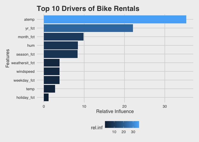
We can visualize the impact of different features on predicting bike rentals using the relative influence provided by GBM. First we can summarize our model then assign these data to a tibble using gbm::summary.gbm() and passing this to the tibble::as_tibble() function.
# summarize model
BikeEffects <- tibble::as_tibble(gbm::summary.gbm(bike_fit_1,
                                         plotit = FALSE))
BikeEffects %>% utils::head()
    ## # A tibble: 6 x 2
    ##   var            rel.inf
    ##
    ## 1 atemp            35.3
    ## 2 yr_fct           22.1
    ## 3 month_fct         9.81
    ## 4 hum               8.41
    ## 5 season_fct        8.35
    ## 6 weathersit_fct    3.91
This creates a new data set with var, a factor variable with the variables in our model, and rel.inf, the relative influence each variable had on our model predictions.
We can then plot the top ten features by impact using ggpplot and our new data frame containing our model summary (BikeEffects).
# plot effects
BikeEffects %>%
  # arrange descending to get the top influencers
  dplyr::arrange(desc(rel.inf)) %>%
  # sort to top 10
  dplyr::top_n(10) %>%
  # plot these data using columns
  ggplot(aes(x = forcats::fct_reorder(.f = var,
                                      .x = rel.inf),
             y = rel.inf,
             fill = rel.inf)) +
  geom_col() +
  # flip
  coord_flip() +
  # format
  scale_color_brewer(palette = "Dark2") +
  theme_fivethirtyeight() +
  theme(axis.title = element_text()) +
  xlab('Features') +
  ylab('Relative Influence') +
  ggtitle("Top 10 Drivers of Bike Rentals")

This let's us know what is being used for selection: Selecting by rel.inf
We can visualize the distribution of our predicted compared with actual bike rentals by predicting these values and plotting the difference.
# Predicted bike rentals
BikeTest$predicted <- base::as.integer(predict(bike_fit_1,
                                         newdata = BikeTest,
                                         n.trees = perf_gbm1))

# plot predicted v actual
ggplot(BikeTest) +
  geom_point(aes(y = predicted,
                 x = cnt,
                 color = predicted - cnt), alpha = 0.7) +
  # add theme
  theme_fivethirtyeight() +
  # strip text
  theme(axis.title = element_text()) +
  # add format to labels
  scale_x_continuous(labels = comma) +
  scale_y_continuous(labels = comma) +
  # add axes/legend titles
  scale_color_continuous(name = "Predicted - Actual",
                         labels = comma) +
  ylab('Predicted Bike Rentals') +
  xlab('Actual Bike Rentals') +
  ggtitle('Predicted vs Actual Bike Rentals')

We can see that our model did a fairly good job predicting bike rentals.
What did we learn?
We learned the ambient temperature is the largest influencer for predicting bike rentals and that rental numbers go down when the temperature reaches ~35 degrees. We can also see holiday (or non-holiday) was not much of an influencer for predicting bike rentals.
- How to model with gradient boosting machine in R - April 9, 2019
- Exploring bike rental behavior using R - April 2, 2019


This is a nice post for learning. Could you please show, how can we see/save the training period simulation data. Then we have the opportunity to calculate different matrix for training period also.
Thank you for this article. Bootstrapping is commonly used with big datasets to help remove the chance of a single training/testing sample skewing the overall result. How would we apply a loop to the model so as to generate the average result after n boostrapping repititions?
Hi Peter
You mention visualizations and graphs, but I only see the code. Is it just me or didn’t you include the graphics?