Exploring bike rental behavior using R
Bikes have become one of the fastest growing modes of city travel which is why it’s no surprise that Lyft and Uber are getting into the two-wheeler game. Lyft’s recent acquisition of Motivate, the largest bike rental company in the world, will compete with Uber’s Jump and Ford’s GoBikes, which have delivered 625,000 and 1.4 million rides in San Francisco, respectively.
The growth of bike rentals presents a unique challenge for both the companies offering these services and the cities responding to the scale of change, particularly in forecasting demand.
The following tutorial will use R and data from Capital Bikeshare available at the UCI Machine Learning Repository to explore bike rentals from 2011 to 2012 in Washington, D.C. We were curious what influenced people renting bikes over the course of the year.
Load packages
# packages --------------------------------------------------
library(tidyverse)
library(rsample) # data splitting
library(randomForest) # basic implementation
library(ranger) # a faster implementation of randomForest
library(caret) # an aggregator package for performing many machine learning models
library(ggthemes)
library(scales)
library(wesanderson)
library(styler)
Import the data
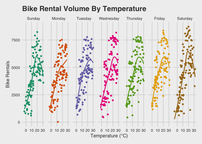
The data we have includes measurements on weather conditions (temperature, humidity, wind speed, etc.), how many bikes were rented, and other seasonal attributes that might influence rentals (i.e. weekdays and holidays). Curiously, riders are more likely to rent a bike after Monday despite temperature and the likelihood increases on Saturdays when temperatures are between 15 to 25 degrees Celsius.
This code will import the daily bike rental data in the data folder.
bike <- readr::read_csv("data/day.csv")Wrangling the data
The following script will wrangling the data and prepare it for modeling. Read through the comments to understand why each step was taken, and how these variables get entered into the visualizations and models.
# WRANGLE ---------------------------------------------------------------
# I like to be overly cautious when it comes to wrangling because all models
# are only as good as the underlying data. This data set came with many
# categorical variables coded numerically, so I am going to create a
# character version of each variable (_chr) and a factor version (_fct).
# Creating a character and factor variable will let me choose which one to
# use for each graph and model.
#
#
#

# this recodes the weekday variable into a character variable
# test
# bike %>%
#   mutate(
#     weekday_chr =
#       case_when(
#         weekday == 0 ~ "Sunday",
#         weekday == 1 ~ "Monday",
#         weekday == 2 ~ "Tuesday",
#         weekday == 3 ~ "Wednesday",
#         weekday == 4 ~ "Thursday",
#         weekday == 5 ~ "Friday",
#         weekday == 6 ~ "Saturday",
#         TRUE ~ "other")) %>%
#     dplyr::count(weekday, weekday_chr) %>%
#     tidyr::spread(weekday, n)

# assign
bike <- bike %>%
  mutate(
    weekday_chr =
      case_when(
        weekday == 0 ~ "Sunday",
        weekday == 1 ~ "Monday",
        weekday == 2 ~ "Tuesday",
        weekday == 3 ~ "Wednesday",
        weekday == 4 ~ "Thursday",
        weekday == 5 ~ "Friday",
        weekday == 6 ~ "Saturday",
        TRUE ~ "other"))

# verify
# bike %>%
#   dplyr::count(weekday, weekday_chr) %>%
#   tidyr::spread(weekday, n)

# Weekdays (factor) ---

# test factor variable
# bike %>%
#   mutate(
#     weekday_fct = factor(x = weekday,
#              levels = c(0,1,2,3,4,5,6),
#              labels = c("Sunday",
#                        "Monday",
#                        "Tuesday",
#                        "Wednesday",
#                        "Thursday",
#                        "Friday",
#                        "Saturday"))) %>%
#   dplyr::count(weekday, weekday_fct) %>%
#   tidyr::spread(weekday, n)

# assign factor variable
bike <- bike %>%
  mutate(
    weekday_fct = factor(x = weekday,
             levels = c(0,1,2,3,4,5,6),
             labels = c("Sunday",
                       "Monday",
                       "Tuesday",
                       "Wednesday",
                       "Thursday",
                       "Friday",
                       "Saturday")))

# verify factor variable
# bike %>%
#   dplyr::count(weekday, weekday_fct) %>%
#   tidyr::spread(weekday, n)


# Holidays ----
# test
# bike %>%
#   mutate(holiday_chr =
#       case_when(
#         holiday == 0 ~ "Non-Holiday",
#         holiday == 1 ~ "Holiday")) %>%
#   dplyr::count(holiday, holiday_chr) %>%
#   tidyr::spread(holiday, n)

# assign
bike <- bike %>%
  mutate(holiday_chr =
      case_when(
        holiday == 0 ~ "Non-Holiday",
        holiday == 1 ~ "Holiday"))

# verify
# bike %>%
#   dplyr::count(holiday, holiday_chr) %>%
#   tidyr::spread(holiday, n)

# test
# bike %>%
#   mutate(
#     holiday_fct = factor(x = holiday,
#              levels = c(0,1),
#              labels = c("Non-Holiday",
#                        "Holiday"))) %>%
#     dplyr::count(holiday, holiday_fct) %>%
#     tidyr::spread(holiday, n)

# assign
bike <- bike %>%
  mutate(
    holiday_fct = factor(x = holiday,
             levels = c(0,1),
             labels = c("Non-Holiday",
                       "Holiday")))

# # verify
# bike %>%
#   dplyr::count(holiday_chr, holiday_fct) %>%
#   tidyr::spread(holiday_chr, n)

# Working days ----
# test
 # bike %>%
 #  mutate(
 #    workingday_chr =
 #      case_when(
 #        workingday == 0 ~ "Non-Working Day",
 #        workingday == 1 ~ "Working Day",
 #        TRUE ~ "other")) %>%
 #    dplyr::count(workingday, workingday_chr) %>%
 #    tidyr::spread(workingday, n)

# assign
 bike <- bike %>%
  mutate(
    workingday_chr =
      case_when(
        workingday == 0 ~ "Non-Working Day",
        workingday == 1 ~ "Working Day",
        TRUE ~ "other"))

 # verify
 # bike %>%
 #    dplyr::count(workingday, workingday_chr) %>%
 #    tidyr::spread(workingday, n)

# test
# bike %>%
#   mutate(
#     workingday_fct = factor(x = workingday,
#              levels = c(0,1),
#              labels = c("Non-Working Day",
#                        "Working Day"))) %>%
#   dplyr::count(workingday, workingday_fct) %>%
#   tidyr::spread(workingday, n)

# assign
bike <- bike %>%
  mutate(
    workingday_fct = factor(x = workingday,
             levels = c(0,1),
             labels = c("Non-Working Day",
                       "Working Day")))

# verify
# bike %>%
#   dplyr::count(workingday_chr, workingday_fct) %>%
#   tidyr::spread(workingday_chr, n)


# Seasons
bike <- bike %>%
  mutate(
    season_chr =
      case_when(
        season == 1 ~ "Spring",
        season == 2 ~ "Summer",
        season == 3 ~ "Fall",
        season == 4 ~ "Winter",
        TRUE ~ "other"
      ))

# test
# bike %>%
#   mutate(
#     season_fct = factor(x = season,
#              levels = c(1, 2, 3, 4),
#              labels = c("Spring",
#                        "Summer",
#                        "Fall",
#                        "Winter"))) %>%
#   dplyr::count(season_chr, season_fct) %>%
#   tidyr::spread(season_chr, n)

# assign
bike <- bike %>%
  mutate(
    season_fct = factor(x = season,
             levels = c(1, 2, 3, 4),
             labels = c("Spring",
                       "Summer",
                       "Fall",
                       "Winter")))

# verify
# bike %>%
#   dplyr::count(season_chr, season_fct) %>%
#   tidyr::spread(season_chr, n)


# Weather situation ----
# test
# bike %>%
#   mutate(
#     weathersit_chr =
#       case_when(
#         weathersit == 1 ~ "Good",
#         weathersit == 2 ~ "Clouds/Mist",
#         weathersit == 3 ~ "Rain/Snow/Storm",
#         TRUE ~ "other")) %>%
#   dplyr::count(weathersit, weathersit_chr) %>%
#   tidyr::spread(weathersit, n)

# assign
bike <- bike %>%
  mutate(
    weathersit_chr =
      case_when(
        weathersit == 1 ~ "Good",
        weathersit == 2 ~ "Clouds/Mist",
        weathersit == 3 ~ "Rain/Snow/Storm"))

# verify
# bike %>%
#   dplyr::count(weathersit, weathersit_chr) %>%
#   tidyr::spread(weathersit, n)

# test
# bike %>%
#   mutate(
#     weathersit_fct = factor(x = weathersit,
#              levels = c(1, 2, 3),
#              labels = c("Good",
#                        "Clouds/Mist",
#                        "Rain/Snow/Storm"))) %>%
#   dplyr::count(weathersit, weathersit_fct) %>%
#   tidyr::spread(weathersit, n)

# assign
bike <- bike %>%
  mutate(
    weathersit_fct = factor(x = weathersit,
                       levels = c(1, 2, 3),
                       labels = c("Good",
                                 "Clouds/Mist",
                                 "Rain/Snow/Storm")))
# verify
# bike %>%
#   dplyr::count(weathersit_chr, weathersit_fct) %>%
#   tidyr::spread(weathersit_chr, n)


# Months ----
# huge shoutout to Thomas Mock over at RStudio for showing me
# lubridate::month() (and stopping my case_when() obsession)
# https://twitter.com/thomas_mock/status/1113105497480183818

# test
# bike %>%
#   mutate(month_ord =
#            lubridate::month(mnth, label = TRUE)) %>%
#   dplyr::count(month_ord, mnth) %>%
#   tidyr::spread(month_ord, n)

# assign
bike <- bike %>%
  mutate(month_ord =
           lubridate::month(mnth, label = TRUE))

# verify
# bike %>%
#   dplyr::count(month_ord, mnth) %>%
#   tidyr::spread(month_ord, n)


# test
# bike %>%
#   mutate(
#     month_fct = factor(x = mnth,
#              levels = c(1, 2, 3, 4, 5, 6, 7, 8, 9, 10, 11, 12),
#              labels = c("January", "February", "March", "April", "May",
#                         "June", "July", "August", "September", "October",
#                         "November", "December"))) %>%
#   dplyr::count(mnth, month_fct) %>%
#   tidyr::spread(month_fct, n)

# assign
bike <- bike %>%
  mutate(
    month_fct = factor(x = mnth,
             levels = c(1, 2, 3, 4, 5, 6, 7, 8, 9, 10, 11, 12),
             labels = c("January", "February", "March", "April", "May",
                        "June", "July", "August", "September", "October",
                        "November", "December")))

# verify
# bike %>%
#   dplyr::count(month_chr, month_fct) %>%
#   tidyr::spread(month_fct, n)

# Year ----
# test
# bike %>%
#   mutate(
#     yr_chr =
#       case_when(
#         yr == 0 ~ "2011",
#         yr == 1 ~ "2012",
#         TRUE ~ "other")) %>%
#     dplyr::count(yr, yr_chr) %>%
#     tidyr::spread(yr, n)

# assign
bike <- bike %>%
  mutate(
    yr_chr =
      case_when(
        yr == 0 ~ "2011",
        yr == 1 ~ "2012"))
# verify
# bike %>%
#     dplyr::count(yr, yr_chr) %>%
#     tidyr::spread(yr, n)

# test
# bike %>%
#   mutate(
#     yr_fct = factor(x = yr,
#              levels = c(0, 1),
#              labels = c("2011",
#                        "2012"))) %>%
#   dplyr::count(yr, yr_fct) %>%
#   tidyr::spread(yr, n)

# assign
bike <- bike %>%
  mutate(
    yr_fct = factor(x = yr,
             levels = c(0, 1),
             labels = c("2011",
                       "2012")))
# verify
# bike %>%
#   dplyr::count(yr_chr, yr_fct) %>%
#   tidyr::spread(yr_chr, n)

# normalize temperatures ----
bike <- bike %>%
  mutate(temp = as.integer(temp * (39 - (-8)) + (-8)))

bike <- bike %>%
  mutate(atemp = atemp * (50 - (16)) + (16))

# ~ windspeed ----
bike <- bike %>%
  mutate(windspeed = as.integer(67 * bike$windspeed))

# ~ humidity ----
bike <- bike %>%
  mutate(hum = as.integer(100 * bike$hum))

# ~ convert to date ----
bike <- bike %>%
  mutate(dteday = as.Date(dteday))

# check df
# bike %>% dplyr::glimpse(78)

# rename the data frame so these don't get confused
BikeData <- bike

# reorganize variables for easier inspection

BikeData <- BikeData %>%
  dplyr::select(
    dplyr::starts_with("week"),
    dplyr::starts_with("holi"),
    dplyr::starts_with("seas"),
    dplyr::starts_with("work"),
    dplyr::starts_with("month"),
    dplyr::starts_with("yr"),
    dplyr::starts_with("weath"),
    dplyr::everything())
If you then dplyr::glimpse(BikeData) you should have the following:
Observations: 731
Variables: 30
$ weekday        <int> 6, 0, 1, 2, 3, 4, 5, 6, 0, 1, 2, 3, 4, 5, 6, 0, 1, 2…
$ weekday_chr    <chr> "Saturday", "Sunday", "Monday", "Tuesday", "Wednesda…
$ weekday_fct    <fct> Saturday, Sunday, Monday, Tuesday, Wednesday, Thursd…
$ holiday        <int> 0, 0, 0, 0, 0, 0, 0, 0, 0, 0, 0, 0, 0, 0, 0, 0, 1, 0…
$ holiday_chr    <chr> "Non-Holiday", "Non-Holiday", "Non-Holiday", "Non-Ho…
$ holiday_fct    <fct> Non-Holiday, Non-Holiday, Non-Holiday, Non-Holiday, …
$ season         <int> 1, 1, 1, 1, 1, 1, 1, 1, 1, 1, 1, 1, 1, 1, 1, 1, 1, 1…
$ season_chr     <chr> "Spring", "Spring", "Spring", "Spring", "Spring", "S…
$ season_fct     <fct> Spring, Spring, Spring, Spring, Spring, Spring, Spri…
$ workingday     <int> 0, 0, 1, 1, 1, 1, 1, 0, 0, 1, 1, 1, 1, 1, 0, 0, 0, 1…
$ workingday_chr <chr> "Non-Working Day", "Non-Working Day", "Working Day",…
$ workingday_fct <fct> Non-Working Day, Non-Working Day, Working Day, Worki…
$ month_ord      <ord> Jan, Jan, Jan, Jan, Jan, Jan, Jan, Jan, Jan, Jan, Ja…
$ month_fct      <fct> January, January, January, January, January, January…
$ yr             <int> 0, 0, 0, 0, 0, 0, 0, 0, 0, 0, 0, 0, 0, 0, 0, 0, 0, 0…
$ yr_chr         <chr> "2011", "2011", "2011", "2011", "2011", "2011", "201…
$ yr_fct         <fct> 2011, 2011, 2011, 2011, 2011, 2011, 2011, 2011, 2011…
$ weathersit     <int> 2, 2, 1, 1, 1, 1, 2, 2, 1, 1, 2, 1, 1, 1, 2, 1, 2, 2…
$ weathersit_chr <chr> "Clouds/Mist", "Clouds/Mist", "Good", "Good", "Good"…
$ weathersit_fct <fct> Clouds/Mist, Clouds/Mist, Good, Good, Good, Good, Cl…
$ instant        <int> 1, 2, 3, 4, 5, 6, 7, 8, 9, 10, 11, 12, 13, 14, 15, 1…
$ dteday         <date> 2011-01-01, 2011-01-02, 2011-01-03, 2011-01-04, 201…
$ mnth           <int> 1, 1, 1, 1, 1, 1, 1, 1, 1, 1, 1, 1, 1, 1, 1, 1, 1, 1…
$ temp           <int> 8, 9, 1, 1, 2, 1, 1, 0, -1, 0, 0, 0, 0, 0, 2, 2, 0, …
$ atemp          <dbl> 28.36325, 28.02713, 22.43977, 23.21215, 23.79518, 23…
$ hum            <int> 80, 69, 43, 59, 43, 51, 49, 53, 43, 48, 68, 59, 47, …
$ windspeed      <int> 10, 16, 16, 10, 12, 6, 11, 17, 24, 14, 8, 20, 20, 8,…
$ casual         <int> 331, 131, 120, 108, 82, 88, 148, 68, 54, 41, 43, 25,…
$ registered     <int> 654, 670, 1229, 1454, 1518, 1518, 1362, 891, 768, 12…
$ cnt            <int> 985, 801, 1349, 1562, 1600, 1606, 1510, 959, 822, 13…
Exploratory data analysis
Here are three options for summarizing the bike table into summary statistics that will give us a better understanding of the underlying distribution for each variable in the BikeData data frame. First, we’ll use the dplyr package.
BikeDplyrSummary <- BikeData %>%
  select(temp, atemp, hum, windspeed, casual, registered, cnt) %>%
  summarise_each(list(
    min = ~min,
    q25 = ~quantile(., 0.25),
    median = ~median,
    q75 = ~quantile(., 0.75),
    max = ~max,
    mean = ~mean,
    sd = ~sd
  )) %>%
  gather(stat, val) %>%
  separate(stat,
           into = c("var", "stat"),
           sep = "_") %>%
  spread(stat, val) %>%
  select(var, min, q25, median, q75, max, mean, sd)

knitr::kable(BikeDplyrSummary)| var | min | q25 | median | q75 | max | mean | sd |
|---|---|---|---|---|---|---|---|
| atemp | 18.68837 | 27.48664 | 32.54892 | 36.69247 | 44.59046 | 32.12804 | 5.540680 |
| casual | 2.00000 | 315.50000 | 713.00000 | 1096.00000 | 3410.00000 | 848.17647 | 686.622488 |
| cnt | 22.00000 | 3152.00000 | 4548.00000 | 5956.00000 | 8714.00000 | 4504.34884 | 1937.211452 |
| hum | 0.00000 | 52.00000 | 62.00000 | 73.00000 | 97.00000 | 62.30643 | 14.242776 |
| registered | 20.00000 | 2497.00000 | 3662.00000 | 4776.50000 | 6946.00000 | 3656.17237 | 1560.256377 |
| temp | -5.00000 | 7.00000 | 15.00000 | 22.00000 | 32.00000 | 14.79617 | 8.546779 |
| windspeed | 1.00000 | 9.00000 | 12.00000 | 15.00000 | 34.00000 | 12.26265 | 5.190293 |
Next, we’ll use the skimr package (which can be found here).
BikeSkimrSummary <- bike %>%
  skimr::skim_to_wide() %>%
  dplyr::select(type,
    variable,
    missing,
    complete,
    min,
    max,
    mean,
    sd,
    median = p50,
    hist)
knitr::kable(BikeSkimrSummary)| type | variable | missing | complete | min | max | mean | sd | median | hist |
|---|---|---|---|---|---|---|---|---|---|
| character | holiday_chr | 0 | 731 | 7 | 11 | NA | NA | NA | NA |
| character | month_chr | 0 | 731 | 3 | 9 | NA | NA | NA | NA |
| character | season_chr | 0 | 731 | 4 | 6 | NA | NA | NA | NA |
| character | weathersit_chr | 0 | 731 | 4 | 15 | NA | NA | NA | NA |
| character | weekday_chr | 0 | 731 | 6 | 9 | NA | NA | NA | NA |
| character | workingday_chr | 0 | 731 | 11 | 15 | NA | NA | NA | NA |
| character | yr_chr | 0 | 731 | 4 | 4 | NA | NA | NA | NA |
| Date | dteday | 0 | 731 | 2011-01-01 | 2012-12-31 | NA | NA | NA | NA |
| factor | holiday_fct | 0 | 731 | NA | NA | NA | NA | NA | NA |
| factor | month_fct | 0 | 731 | NA | NA | NA | NA | NA | NA |
| factor | season_fct | 0 | 731 | NA | NA | NA | NA | NA | NA |
| factor | weathersit_fct | 0 | 731 | NA | NA | NA | NA | NA | NA |
| factor | weekday_fct | 0 | 731 | NA | NA | NA | NA | NA | NA |
| factor | workingday_fct | 0 | 731 | NA | NA | NA | NA | NA | NA |
| factor | yr_fct | 0 | 731 | NA | NA | NA | NA | NA | NA |
| integer | casual | 0 | 731 | NA | NA | 848.18 | 686.62 | 713 | ▇▇▅▂▁▁▁▁ |
| integer | cnt | 0 | 731 | NA | NA | 4504.35 | 1937.21 | 4548 | ▂▅▅▇▇▅▅▂ |
| integer | holiday | 0 | 731 | NA | NA | 0.029 | 0.17 | 0 | ▇▁▁▁▁▁▁▁ |
| integer | hum | 0 | 731 | NA | NA | 62.31 | 14.24 | 62 | ▁▁▁▃▇▇▅▂ |
| integer | instant | 0 | 731 | NA | NA | 366 | 211.17 | 366 | ▇▇▇▇▇▇▇▇ |
| integer | mnth | 0 | 731 | NA | NA | 6.52 | 3.45 | 7 | ▇▅▇▃▅▇▅▇ |
| integer | registered | 0 | 731 | NA | NA | 3656.17 | 1560.26 | 3662 | ▁▅▅▆▇▅▃▃ |
| integer | season | 0 | 731 | NA | NA | 2.5 | 1.11 | 3 | ▇▁▇▁▁▇▁▇ |
| integer | temp | 0 | 731 | NA | NA | 14.8 | 8.55 | 15 | ▁▅▇▇▆▆▇▂ |
| integer | weathersit | 0 | 731 | NA | NA | 1.4 | 0.54 | 1 | ▇▁▁▅▁▁▁▁ |
| integer | weekday | 0 | 731 | NA | NA | 3 | 2 | 3 | ▇▇▇▇▁▇▇▇ |
| integer | windspeed | 0 | 731 | NA | NA | 12.26 | 5.19 | 12 | ▂▇▇▆▂▁▁▁ |
| integer | workingday | 0 | 731 | NA | NA | 0.68 | 0.47 | 1 | ▃▁▁▁▁▁▁▇ |
| integer | yr | 0 | 731 | NA | NA | 0.5 | 0.5 | 1 | ▇▁▁▁▁▁▁▇ |
| numeric | atemp | 0 | 731 | NA | NA | 32.13 | 5.54 | 32.55 | ▁▅▇▇▇▇▆▁ |
Finally, we’ll use the mosaic package (which can be found here).
BikeMosaicInspect <- mosaic::inspect(BikeData)
# categorical
knitr::kable(BikeMosaicInspect$categorical)| name | class | levels | n | missing | distribution |
|---|---|---|---|---|---|
| weekday_chr | character | 7 | 731 | 0 | Monday (14.4%), Saturday (14.4%) … |
| weekday_fct | factor | 7 | 731 | 0 | Sunday (14.4%), Monday (14.4%) … |
| holiday_chr | character | 2 | 731 | 0 | Non-Holiday (97.1%), Holiday (2.9%) |
| holiday_fct | factor | 2 | 731 | 0 | Non-Holiday (97.1%), Holiday (2.9%) |
| workingday_chr | character | 2 | 731 | 0 | Working Day (68.4%) … |
| workingday_fct | factor | 2 | 731 | 0 | Working Day (68.4%) … |
| season_chr | character | 4 | 731 | 0 | Fall (25.7%), Summer (25.2%) … |
| season_fct | factor | 4 | 731 | 0 | Fall (25.7%), Summer (25.2%) … |
| weathersit_chr | character | 3 | 731 | 0 | Good (63.3%), Clouds/Mist (33.8%) … |
| weathersit_fct | factor | 3 | 731 | 0 | Good (63.3%), Clouds/Mist (33.8%) … |
| month_chr | character | 12 | 731 | 0 | August (8.5%), December (8.5%) … |
| month_fct | factor | 12 | 731 | 0 | January (8.5%), March (8.5%) … |
| yr_chr | character | 2 | 731 | 0 | 2012 (50.1%), 2011 (49.9%) |
| yr_fct | factor | 2 | 731 | 0 | 2012 (50.1%), 2011 (49.9%) |
# date
knitr::kable(BikeMosaicInspect$Date)
| name | class | first | last | min_diff | max_diff | n | missing |
|---|---|---|---|---|---|---|---|
| dteday | Date | 2011-01-01 | 2012-12-31 | 1 days | 1 days | 731 | 0 |
# quantitative
knitr::kable(BikeMosaicInspect$quantitative)
| name | class | min | Q1 | median | Q3 | max | mean | sd | n | missing |
|---|---|---|---|---|---|---|---|---|---|---|
| instant | integer | 1.00000 | 183.50000 | 366.00000 | 548.50000 | 731.00000 | 366.0000000 | 211.1658116 | 731 | 0 |
| season | integer | 1.00000 | 2.00000 | 3.00000 | 3.00000 | 4.00000 | 2.4965800 | 1.1108071 | 731 | 0 |
| yr | integer | 0.00000 | 0.00000 | 1.00000 | 1.00000 | 1.00000 | 0.5006840 | 0.5003419 | 731 | 0 |
| mnth | integer | 1.00000 | 4.00000 | 7.00000 | 10.00000 | 12.00000 | 6.5198358 | 3.4519128 | 731 | 0 |
| holiday | integer | 0.00000 | 0.00000 | 0.00000 | 0.00000 | 1.00000 | 0.0287278 | 0.1671547 | 731 | 0 |
| weekday | integer | 0.00000 | 1.00000 | 3.00000 | 5.00000 | 6.00000 | 2.9972640 | 2.0047869 | 731 | 0 |
| workingday | integer | 0.00000 | 0.00000 | 1.00000 | 1.00000 | 1.00000 | 0.6839945 | 0.4652334 | 731 | 0 |
| weathersit | integer | 1.00000 | 1.00000 | 1.00000 | 2.00000 | 3.00000 | 1.3953488 | 0.5448943 | 731 | 0 |
| temp | integer | -5.00000 | 7.00000 | 15.00000 | 22.00000 | 32.00000 | 14.7961696 | 8.5467794 | 731 | 0 |
| atemp | numeric | 18.68837 | 27.48664 | 32.54892 | 36.69247 | 44.59046 | 32.1280356 | 5.5406801 | 731 | 0 |
| hum | integer | 0.00000 | 52.00000 | 62.00000 | 73.00000 | 97.00000 | 62.3064295 | 14.2427756 | 731 | 0 |
| windspeed | integer | 1.00000 | 9.00000 | 12.00000 | 15.00000 | 34.00000 | 12.2626539 | 5.1902926 | 731 | 0 |
| casual | integer | 2.00000 | 315.50000 | 713.00000 | 1096.00000 | 3410.00000 | 848.1764706 | 686.6224883 | 731 | 0 |
| registered | integer | 20.00000 | 2497.00000 | 3662.00000 | 4776.50000 | 6946.00000 | 3656.1723666 | 1560.2563770 | 731 | 0 |
| cnt | integer | 22.00000 | 3152.00000 | 4548.00000 | 5956.00000 | 8714.00000 | 4504.3488372 | 1937.2114516 | 731 | 0 |
Exploring the impact of weather conditions on bike rentals
Unlike ride-share passengers, bikers are vulnerable to weather conditions, and this might impact their likelihood of choosing a bike over other transportation options. If weather conditions are influential in transportation decisions, we would expect to see relationships between the number of bike rentals and weather features including temperature, humidity and wind speed. Let’s explore.
# ~ rentals by temperature ----
ggRentalsByTemp <- BikeData %>%
  ggplot(aes(y = cnt,
                 x = temp,
                 color = weekday_fct)) +
  geom_point(show.legend = FALSE) +
  geom_smooth(se = FALSE,
              show.legend = FALSE) +
  facet_grid(~weekday_fct) +
  scale_color_brewer(palette = "Dark2") +
  theme_fivethirtyeight() +
  theme(axis.title = element_text()) +
  ylab("Bike Rentals") +
  xlab("Temperature (°C)") +
  ggtitle("Bike Rental Volume By Temperature")
ggRentalsByTemp
The output below is R’s way of telling us how the best-fit line is being drawn through each set of data. This fits a LOESS local polynomial regression to the data.
`geom_smooth()` using method = 'loess' and formula 'y ~ x'
We would also expect windier conditions to negatively impact bike rentals. Let’s analyze the data.
# ggRentalVolByWindSpeed ----
ggRentalVolByWindSpeed <- ggplot(bike) +
  geom_point(aes(y = cnt,
                 x = windspeed,
                 color = weekday_fct),
             show.legend = FALSE) +
  facet_grid(~weekday_fct) +
  scale_color_brewer(palette = "Dark2") +
  theme_fivethirtyeight() +
  theme(axis.title = element_text()) +
  ylab("Bike Rentals") +
  xlab("Windspeed") +
  ggtitle("Rental Volume By Windspeed")
ggRentalVolByWindSpeed
Exploring the impact of holidays on bike rental volume
Holidays might influence bike riders in different ways. For instance, we can think of holidays as increasing opportunities for bike riders to enjoy being on the road with fewer drivers, since typically fewer people drive on holidays. We could also consider a situation where bike enthusiasts only prefer to ride their bikes on summer or spring holidays (considering the information we’ve learned about the influences of weather conditions on bike rentals).
ggRentalVolByHoliday <- ggplot(BikeData) +
  geom_density(aes(x = cnt,
                   fill = holiday_chr),
                   alpha = 0.2) +
  scale_fill_brewer(palette = "Paired") +

  theme_fivethirtyeight() +
  theme(axis.title = element_text()) +
  labs(title = "Bike Rental Density By Holiday",
               fill = "Holiday",
               x = "Average Bike Rentals",
               y = "Density")

ggRentalVolByHoliday
With both Lyft and Uber preparing for IPOs this year and total rideshares for each company hitting one billion and 10 billion rides, respectively, the pace of transportation disruption in cities across the country seems to be increasing. How this evolution will impact greener forms of transportation like bikes will in part be determined by the ability of companies and cities to plan and execute on accommodating demand. Learning to forecast this shift will be an important skill for most everyone involved.
Edit 2019-04-03: The code for this post is available here on Github.
- How to model with gradient boosting machine in R - April 9, 2019
- Exploring bike rental behavior using R - April 2, 2019


Fantastic!
Hi, fantastic work. I have one question though: When I try to run your code I get the following error:
Error: Column `temp_min` is of unsupported type function.
I can work around that with unclass() first, but then I get a second error message:
message: `select()` doesn’t handle lists.
class: `rlang_error`
backtrace:
1. base::lapply(., unclass)
9. dplyr::select(…)
Call `rlang::last_trace()` to see the full backtrace
> rlang::last_trace()
x
1. \-`%>%`(…)
2. +-base::withVisible(eval(quote(`_fseq`(`_lhs`)), env, env))
3. \-base::eval(quote(`_fseq`(`_lhs`)), env, env)
4. \-base::eval(quote(`_fseq`(`_lhs`)), env, env)
5. \-`_fseq`(`_lhs`)
6. \-magrittr::freduce(value, `_function_list`)
7. \-function_list[[i]](value)
8. +-dplyr::select(…)
9. \-dplyr:::select.list(…)
Is this a problem with different versions of R?