Deciding whether to reelect President Donald Trump isn’t the only choice Americans will have to make when they head to the voting booths this November. More than 5,000 state lawmakers are up for election and that means voting in legislators that will determine how Congressional and state House and Senate districts will be redrawn in the near future.

“The reins of political power in the U.S. for the next decade could be determined in this year’s elections — not necessarily by who wins the presidency, but by thousands of lower-profile contests for state legislative seats across the country,” wrote the AP’s David Lieb earlier this month.

Redistricting usually favors one political party over another and is therefore an area of fierce debate. Last summer, gerrymandering, as it’s often called, reached the Supreme Court. As NPR put it, the court ruled that “partisan redistricting is a political question — not reviewable by federal courts — and that those courts can’t judge if extreme gerrymandering violates the Constitution. The ruling puts the onus on the legislative branch, and on individual states, to police redistricting efforts.”

Researchers have a role in studying – if not policing – these efforts, too. During the summer, I worked for the Voting Rights Data Institute (VRDI), a six-week summer program of the Metric Geometry and Gerrymandering Group (MGGG). MGGG is a Boston-based working group led by Moon Duchin of Tufts University and Justin Solomon of MIT, whose mission is to study applications of geometry and computing to U.S. redistricting.

How we use math to determine hundreds of possible redistricting plans

At the Voting Rights Data Institute, one of our main tasks was to generate a large ensemble of districting plans for analysis and evaluation. The mathematical sampling technique we used is called Markov chain, a model designed to examine a sequence of possible events based on probabilities.

Our Markov chain sampling process takes into account basic constraints such as population equality, contiguity, and compactness. Population equality means that districts in a state have to have nearly equal populations; contiguity means that districts in a state have to be physically adjacent; and in short, compactness is a measure of how reasonably shaped districts are, although there exist many measures of compactness among mathematicians and legislators.

Why are we using Markov chain? Well, it turns out there are many, many ways to make districts in a state. For example, in Minnesota, there are 6,156,723,718,225,577,984 different ways to make 67 state Senate districts. It is therefore impossible to explore all these plans at once. Markov chain – a random walk with no memory – enables us to sample efficiently from the subspace of plans with prescribed properties.

To construct an ensemble of plans with a Markov chain, we begin with an initial districting plan, then the Markov chain applies a randomized algorithm to each newly generated plan. The defining property of a Markov chain is that the probability of observing each possible plan next, at a particular iteration, is determined only by the plan at the previous iteration. Our proposal methods all modify an existing plan by randomly choosing a set of its units for which to switch the districting assignment.

For this article, I will be using two designs of Markov chains to build ensembles.

• Single edge flip (“Flip“). At each step in the Markov chain, we (uniformly) randomly select a pair of adjacent census blocks that are assigned to different districts, then (uniformly) randomly change the assignment of one of the blocks so that they match.

• Recombination (“ReCom“). At each step, we (uniformly) randomly select a pair of adjacent districts and merge all of their blocks into a single unit. Then, we generate a spanning tree for the blocks of the merged unit with the Kruskal/Karger algorithm. Finally, we cut an edge of the tree at random, checking that this separates the region into two new districts that are population balanced to within 2% of ideal district size. Figure 1 shows an illustration of this process.

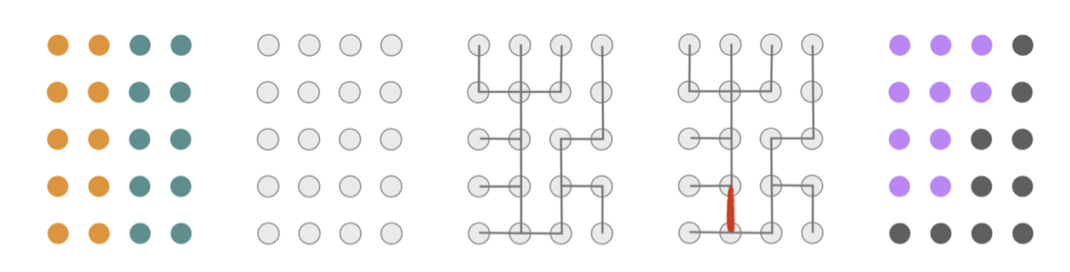
(The descriptions of Markov chain, “Flip,” “Recom” and above figure are taken from the report “Recombination: A family of Markov chains for redistricting” by MGGG.)

Building ensembles

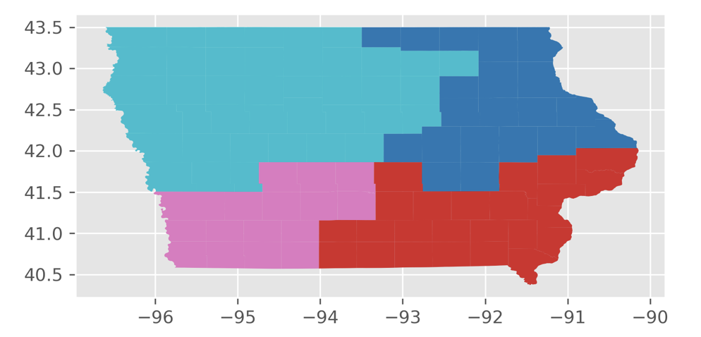
In this article, I will be using the Iowa shapefile to build ensembles.

Here’s a picture of the Iowa shapefile. This shapefile was obtained from the U.S. Census Bureau and processed by MGGG. It is at the county level.

To build the ensemble, I started with the initial plan by putting every county into the congressional district they currently belong to.

I applied three constraints onto the Markov chain. First, I kept the population of each district to be within a maximum of 2 percent deviation from the population of each district of the original plan. Second, to keep districts about as compact as the original plan, I bounded the number of cut edges at 2 times the number of cut edges of the initial plan. (The number of cut edges is a measure of compactness because a district that is reasonably shaped will not need many edges to be cut to separate them from the rest of the state.) Last, I applied a third constraint to make sure that each district in the plan is contiguous.

Here’s an animation of the first 30 plans generated by “ReCom.”

Here’s an animation of the first 30 plans generated by “Flip.”

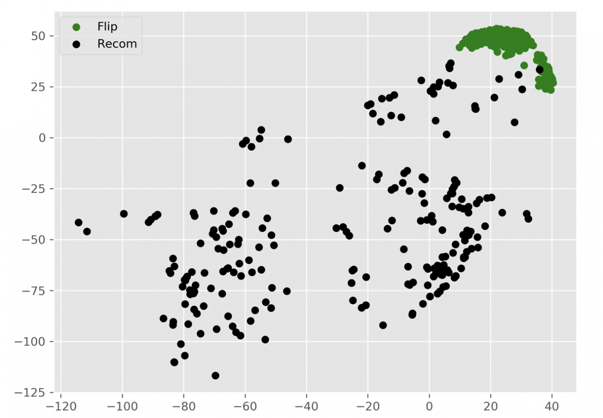
We found that the “ReCom” method is able to explore a much larger space of possible plans than “Flip”. To visualize this, I generated 250 plans each for “ReCom” and “Flip”. I then used multidimensional scaling (MDS) – a method that visualizes the level of similarity of individual cases of a dataset – to map the original high dimensional space of districting plans onto a two-dimensional embedded space.

At the end of my research experience, my knowledge of Markov chain and multidimensional scaling helped me coauthor a paper on arXiv, “Geometry of Graph Partitions via Optimal Transport.”

In this paper, my coauthors and I explored ways to find minimum-cost network flows between census dual graphs, and used this to quantify the notion of similarity or difference between two districting plans to determine how “diverse” a sample of districting plans might be.

https://twitter.com/zschutzy/status/1186998578142732289

We hope this paper can inspire people to expand on the theory and applications of distances between graph partitions.

My full code for running Markov chains is below. (You can find the code that are stored in files “iowa”, “settings” and “wasserplan” here, here and here.)

# creating 250 “ReCom” partitions from GerryChain

import yaml
from iowa import *

with open('settings.yaml', 'r') as stream:
    settings = yaml.load(stream)

graph = Graph.from_file(settings['data_path_shp'], reproject=False)

recom_partitions = MC_sample(graph, settings, save_part=False) 

df = gpd.read_file(settings['data_path_shp']) # reading shapefile

# plotting ReCom partitions [0] to [29] with ggplot

%config InlineBackend.figure_formats = ['svg']
plt.style.use('ggplot')
fig=recom_partitions[29].plot(df).get_figure()
fig.savefig('ReCom29.png',dpi=300, bbox_inches='tight')

# creating 250 “Flip” partitions from GerryChain (we can do this by changing “recom” to “flip” in the “settings” file)

with open('settings.yaml', 'r') as stream:
    settings = yaml.load(stream)

graph = Graph.from_file(settings['data_path_shp'], reproject=False)

flip_partitions = MC_sample(graph, settings, save_part=False)

# plotting Flip partitions [0] to [29] with ggplot

fig=flip_partitions[29].plot(df).get_figure()
fig.savefig('Flip29.png',dpi=300, bbox_inches='tight')

new_partitions=recom_partitions+flip_partitions

# create pairwise distance matrix for MDS visualizations

import wasserplan

Distance_matrix=np.zeros((500,500))

for i in range(500):
    for j in range(i+1,500):
        Distance_matrix[i][j] = wasserplan.Pair(new_partitions[i],new_partitions[j]).distance
        Distance_matrix[j][i] = Distance_matrix[i][j]

# MDS visualization of ReCom and Flip partitions in one figure

from sklearn.manifold import MDS

mds = MDS(n_components=2, metric=True, n_init=4, max_iter=300, verbose=0, eps=0.001, n_jobs=None, random_state=None, dissimilarity='euclidean')

pos=mds.fit(Distance_matrix).embedding_


X_MDS=[]
Y_MDS=[]
for i in range(500):
    X_MDS.append(pos[i][0])
Y_MDS.append(pos[i][1])


import matplotlib.pyplot as plt

fig=plt.figure(figsize=(8,6))
plt.scatter(X_MDS[250:500],Y_MDS[250:500],color=['green'])
plt.scatter(X_MDS[0:250],Y_MDS[0:250],color=['black'])
plt.legend(('Flip', 'Recom'), loc='upper left')
fig.savefig('recom_flip.png',dpi=300, bbox_inches='tight')