Getting started with stringr for textual analysis in R
stringr package from the tidyverse. The datasets being used are being analyzed as part of the Reinventing Local TV News Project at Northeastern University’s School of Journalism. The full RMarkdown file can be found here.Load the Packages
Start by loading the packages we will be using in this tutorial.
library(dplyr) # Data wrangling, glimpse(75) and tbl_df().

library(ggplot2) # Visualise data.
library(lubridate) # Dates and time.
library(readr) # Efficient reading of CSV data.
library(stringr) # String operations.
library(tibble) # Convert row names into a column.
library(tidyr) # Prepare a tidy dataset, gather().
library(magrittr) # Pipes %>%, %T>% and equals(), extract().
library(tidyverse) # all tidyverse packages
library(mosaic) # favstats and other summary functions
library(fs) # file management functions
library(forcats) # manipulate data for visualization
library(cowplot) # visualization
library(stringi) # more strings
library(tidytext) # tidying text data for analysis
library(maps) # maps for us.cities
Load the Data
We will be using 6 months of news article data from ABC7NY in New York and KCRA in California, spanning July 18 to January 16 (headline, date-time, teaser, url). All times are Eastern Standard Time. You can find the files here: abc7ny.csv and kcra.csv.
Abc7 <- read_csv("Data/abc7ny.csv")
Kcra <- read_csv("Data/kcra.csv")
Inspect the data sets
Take a quick look at each data set with dplyr::glimpse(75)
Abc7 %>% glimpse(78)Observations: 9,745
Variables: 6
$ datetime <chr> "July 18, 2017 at 03:41PM", "July 18, 2017 at 03:55PM",...
$ headline <chr> "9-year-old boy wants to thank every cop in the U.S. wi...
$ url <chr> "http://abc7ny.com/news/donut-boy-wants-to-thank-every-...
$ teaser <chr> "Tyler Carach, a 9-year-old boy from Florida, wants to ...
$ feed_name <chr> "abc7ny.com RSS Feed", "abc7ny.com RSS Feed", "abc7ny.c...
$ feed_url <chr> "http://abc7ny.com/feed", "http://abc7ny.com/feed", "ht...Kcra %>% glimpse(78)Observations: 13,020
Variables: 6
$ datetime <chr> "July 18, 2017 at 03:56PM", "July 18, 2017 at 03:58PM",...
$ headline <chr> "Woman says product intended for wasps trapped 7 birds ...
$ url <chr> "http://www.kcra.com/article/woman-says-product-intende...
$ teaser <chr> "The customer's Facebook post has been shared thousands...
$ feed_name <chr> "KCRA Top Stories", "KCRA Top Stories", "KCRA Top Stori...
$ feed_url <chr> "http://www.kcra.com", "http://www.kcra.com", "http://w...We can see these data frames contain the same variables, but if we had many, many columns we could use base::identical()and base::names() to test if the columns are the same.
base::identical(names(Abc7), names(Kcra))[1] TRUECombine the data sets
We want to combine these data sets into a single data frame NewsData. As with most operations in R, there are multiple ways to approach combining data frames. I prefer to use dplyr for merging and joining because 1) the functions are fast and efficient and 2) the arguments are somewhat intuitive.
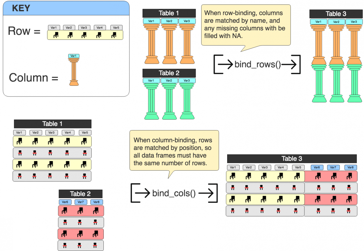
I say somewhat because dplyr::bind_rows() sticks two data frames together top-to-bottom, and dplyr::bind_cols() puts two data frames together side-by-side. If you look at the figure below, you can see what I mean. Combining two data frames together top-to-bottom means the data gets added into the matched columns (and un-matched columns get filled with NA).
But if I want to combine data frames together side-by-side, they will be matched on their row position (so I would need to make sure the same number of rows are in each data frame).
NOTE: The tiny object in the rows are chairs, because for some reason, whenever I think of rows, I think of a row of chairs. The same goes for columns (except I think about a Roman pillar).
Which one do I want to use?
I can see from the code chunks above that both data frames have identical column names, but an unequal number of rows. This makes dplyr::bind_rows() the correct option. I might want to separate each data frame again later, so including an ID (like data_id) that allows me to see what data set each headline originally came from is a good idea. Fortunately, there is an argument in dplyr::bind_rows() for including an id (.id =).
Before I start executing functions, I should think about to expect in NewsData. The Abc7 data frame has 9,745 and 6 variables, and Kcra has 13,020 observations and 6 variables. If I use dplyr::bind_rows(), I’m expecting a data frame with the sum of all observations (i.e. 22,765) and 6 variables.
# test
dplyr::bind_rows(Abc7, Kcra, .id = "data_id") %>%
dplyr::count(data_id)|
data_id
<chr>
|
n
<int>
|
|---|---|
| 1 | 9745 |
| 2 | 13020 |
NOTE: I’m going to introduce a little sequence I go through for most data manipulation tasks. It includes three steps: 1) test, 2) assign, and 3) verify. These steps are for making sure I am getting what I expect from each task. In the test step, I set up some way of verifying the function or pipeline is doing what I want. For this example, I used dplyr::count() to see if "data_id" is the new data frame and if it can distinguish the original data sets.
Now I will assign the new variables to NewsData and verify it gives the same information.
# assign
NewsData <- dplyr::bind_rows(Abc7, Kcra, .id = "data_id")
# verify
NewsData %>%
dplyr::count(data_id)|
data_id
<chr>
|
n
<int>
|
|---|---|
| 1 | 9745 |
| 2 | 13020 |
Great! I just need to remember that 1 is the id for Abc7 and 2 is the id for Kcra. Now I can start with the string manipulations.
NewsData %>%
    glimpse(75)
Observations: 22,765
Variables: 7
$ data_id <chr> "1", "1", "1", "1", "1", "1", "1", "1", "1", "1", "1...
$ datetime <chr> "July 18, 2017 at 03:41PM", "July 18, 2017 at 03:55P...
$ headline <chr> "9-year-old boy wants to thank every cop in the U.S....
$ url <chr> "http://abc7ny.com/news/donut-boy-wants-to-thank-eve...
$ teaser <chr> "Tyler Carach, a 9-year-old boy from Florida, wants ...
$ feed_name <chr> "abc7ny.com RSS Feed", "abc7ny.com RSS Feed", "abc7n...
$ feed_url <chr> "http://abc7ny.com/feed", "http://abc7ny.com/feed", ...String manipulation with base R
There are a few functions in base R that come in handy when dealing with strings. These first functions we will cover are basic, but they introduce important concepts like how strings are printed, and the kinds of manipulations that are possible with R. I’ll demo these by taking the first five lines of the headline column and putting it into it’s object (headlines_var) using dplyr::select() and Matrix::head().
headlines_var <- NewsData %>%
    dplyr::select(headline) %>%
    Matrix::head(5)
Testing Character Strings
The base functions in R takes a character vector, so the first thing I’ll need to do is test and see if headlines_var satisfies that condition. I can do this with base::is.character().
base::is.character(headlines_var)[1] FALSEFALSE!?!? But this looked like a character vector when I used dplyr::glimpse(75) above. What kind of object this isheadlines_var?
I can test that with base::typeof().
base::typeof(headlines_var)[1] "list"Ahhhh headlines_var is a list. This means I’ll need to use base::unlist() to convert the headlines_var list to a character vector.
headlines_var <- headlines_var %>% base::unlist()
base::is.character(headlines_var)
[1] TRUENOTE: Other options for converting objects to strings include base::is.character() and base::toString().
I’ll take a look at this vector and see what the contents look like with utils::str().
headlines_var %>% utils::str() Named chr [1:5] "9-year-old boy wants to thank every cop in the U.S. with doughnuts" ...
- attr(*, "names")= chr [1:5] "headline1" "headline2" "headline3" "headline4" ...We can see the unlist() function retains the "names" attribute in the headlines_var vector.
headlines_var headline1
"9-year-old boy wants to thank every cop in the U.S. with doughnuts"
headline2
"10-year-old boy critical after being struck by boat propeller on Long Island"
headline3
"10-year-old boy critical after Long Island boating accident"
headline4
"American Airlines mechanic marks record-breaking 75 years with company"
headline5
"12-year-old girl pulled from surf in Sandy Hook dies" Removing characters
I can see from the contents of headlines_var that it is a vector with all five headlines. I’ll demonstrate the base::sub()function by removing the - characters.
base::sub(pattern = "-", replacement = " ", x = headlines_var) headline1
"9 year-old boy wants to thank every cop in the U.S. with doughnuts"
headline2
"10 year-old boy critical after being struck by boat propeller on Long Island"
headline3
"10 year-old boy critical after Long Island boating accident"
headline4
"American Airlines mechanic marks record breaking 75 years with company"
headline5
"12 year-old girl pulled from surf in Sandy Hook dies" The first pass with base::sub() only finds the first instance of - and replaces it with a blank space " ". If I want to remove ALL instances of -, I can use base::gsub().
base::gsub(pattern = "-", replacement = " ", x = headlines_var) headline1
"9 year old boy wants to thank every cop in the U.S. with doughnuts"
headline2
"10 year old boy critical after being struck by boat propeller on Long Island"
headline3
"10 year old boy critical after Long Island boating accident"
headline4
"American Airlines mechanic marks record breaking 75 years with company"
headline5
"12 year old girl pulled from surf in Sandy Hook dies" Another option for replacing every instance of a character is base::chartr(), but this requires that the old argument is the same length of the new argument (otherwise you will see 'old' is longer than 'new').
base::chartr(old = "-", new = " ", x = headlines_var) headline1
"9 year old boy wants to thank every cop in the U.S. with doughnuts"
headline2
"10 year old boy critical after being struck by boat propeller on Long Island"
headline3
"10 year old boy critical after Long Island boating accident"
headline4
"American Airlines mechanic marks record breaking 75 years with company"
headline5
"12 year old girl pulled from surf in Sandy Hook dies" Pasting
Whenever you need to combine or “stick” string elements together, you can either use base::paste() or base::paste0(). For example, if I wanted to combine all of these headlines into a single, long, character vector, I could use the following
base::paste(headlines_var, collapse = "; ")[1] "9-year-old boy wants to thank every cop in the U.S. with doughnuts; 10-year-old boy critical after being struck by boat propeller on Long Island; 10-year-old boy critical after Long Island boating accident; American Airlines mechanic marks record-breaking 75 years with company; 12-year-old girl pulled from surf in Sandy Hook dies"Or if I wanted to combine all the headlines but not include any whitespace between the characters, I could use base::paste0()
base::paste0(headlines_var, sep = "", collapse = "; ")[1] "9-year-old boy wants to thank every cop in the U.S. with doughnuts; 10-year-old boy critical after being struck by boat propeller on Long Island; 10-year-old boy critical after Long Island boating accident; American Airlines mechanic marks record-breaking 75 years with company; 12-year-old girl pulled from surf in Sandy Hook dies"Printing
I typically use RStudio Notebooks, so I like to have some flexibility with my printing options. There are a few base R printing options you should know for printing strings (or anything) to the R console.
If you want to see the results of a vector printed without quotes, use base::noquote()
base::noquote(headlines_var) headline1
9-year-old boy wants to thank every cop in the U.S. with doughnuts
headline2
10-year-old boy critical after being struck by boat propeller on Long Island
headline3
10-year-old boy critical after Long Island boating accident
headline4
American Airlines mechanic marks record-breaking 75 years with company
headline5
12-year-old girl pulled from surf in Sandy Hook dies Another option is base::cat(). This also comes with a sep = argument.
base::cat(headlines_var, sep = ", ")9-year-old boy wants to thank every cop in the U.S. with doughnuts, 10-year-old boy critical after being struck by boat propeller on Long Island, 10-year-old boy critical after Long Island boating accident, American Airlines mechanic marks record-breaking 75 years with company, 12-year-old girl pulled from surf in Sandy Hook diesThe stringr package
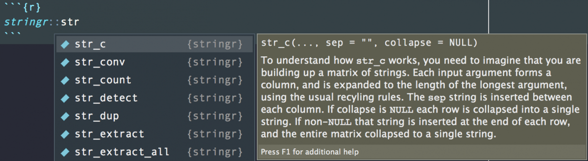
The tidyverse comes with stringr, a handy package for handling string manipulations. You can find it on the tidyversewebsite or you can read about here in R for Data Science.
stringr (like other packages in the tidyverse) is very convenient because all of the functions have a common prefix, str_
 p
p
Everything we just did with base R is possible with stringr, so I’m going to go through some of this package’s lesser-known functions.
Changing case
It’s often useful to convert the entire corpus of text to lowercase so future string matching is a little easier. I can do this by changing the case of headlines and storing it in a new variable headline_low using stringr::str_to_lower() and dplyr::mutate().
NOTE: I’m going to perform the remaining functions with the NewsData data frame (because that is the preferred object in the tidyverse).
NewsData %>%
    dplyr::mutate(headline_low = stringr::str_to_lower(headline)) %>%
    dplyr::select(headline, headline_low) %>%
head(5)|
headline
<chr>
|
|
|---|---|
| 9-year-old boy wants to thank every cop in the U.S. with doughnuts | |
| 10-year-old boy critical after being struck by boat propeller on Long Island | |
| 10-year-old boy critical after Long Island boating accident | |
| American Airlines mechanic marks record-breaking 75 years with company | |
| 12-year-old girl pulled from surf in Sandy Hook dies |
Then again, these are headlines, so maybe we want another variable that converts all headlines to Title Case using stringr::str_to_title().
NewsData %>%
    dplyr::mutate(headline_title = stringr::str_to_title(headline)) %>%
    dplyr::select(headline, headline_title) %>%
head(5)|
headline
<chr>
|
|
|---|---|
| 9-year-old boy wants to thank every cop in the U.S. with doughnuts | |
| 10-year-old boy critical after being struck by boat propeller on Long Island | |
| 10-year-old boy critical after Long Island boating accident | |
| American Airlines mechanic marks record-breaking 75 years with company | |
| 12-year-old girl pulled from surf in Sandy Hook dies |
Finding words
I might also curious about the first few words in the teaser associated with each headline. Let’s assume I want to see the frequency of each word by news feed (or data_id). I can use the stringr::word() function to extract the first three words and store it in a new variable teaser_3_words.
# test
NewsData %>%
    dplyr::mutate(teaser_3_words = stringr::word(NewsData$teaser, 1, 3)) %>%
    count(teaser_3_words, sort = TRUE) %>%
head(10)|
teaser_3_words
<chr>
|
n
<int>
|
|---|---|
| President Donald Trump | 216 |
| Get weather conditions | 132 |
| Police say the | 114 |
| KCRA 3 Weather | 107 |
| Here and Now: | 102 |
| Good morning, Northern | 87 |
| The incident happened | 77 |
| The fire broke | 65 |
| Authorities say the | 43 |
| The New York | 42 |
This looks like it’s working, so I’ll assign teaser_3_words to the NewsData data frame.
NewsData <- NewsData %>%
    dplyr::mutate(teaser_3_words = stringr::word(NewsData$teaser, 1, 3))
Now I can verify this new variable is behaving the way it should by using the same dplyr::count() function above.
NewsData %>%
    dplyr::count(teaser_3_words, sort = TRUE) %>%
utils::head(10)|
teaser_3_words
<chr>
|
n
<int>
|
|---|---|
| President Donald Trump | 216 |
| Get weather conditions | 132 |
| Police say the | 114 |
| KCRA 3 Weather | 107 |
| Here and Now: | 102 |
| Good morning, Northern | 87 |
| The incident happened | 77 |
| The fire broke | 65 |
| Authorities say the | 43 |
| The New York | 42 |
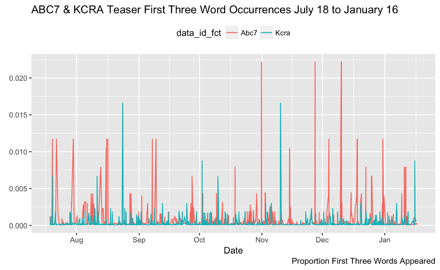
Sometimes I like to verify a new variable using a visualization instead of a table. I find it helpful to think of the data I am manipulating as a distribution (or shape) instead of just a set of numbers in a table. A figure has more attributes I can think about (shape, size, color, position, etc.), where a table just has lines and text.
For example, when I created teaser_3_words with the first three words from the teaser, I was thinking about how those words might vary by station (ABC7NY or KCRA) over time. I assume there is some overlap in teaser_3_words between these stations. I can see this if I run dplyr::distinct() and base::nrow().
NewsData %>%
    dplyr::distinct(teaser_3_words) %>%
    base::nrow()
[1] 15415If there are 15415 distinct teaser_3_words and 22765 observations in NewsData, I can safely assume there is some overlap between these two stations.
Create a visualization with a pipeline
If I want to visualize this, I need to add a column to the NewsData data frame that has the results from dplyr::count(). This is possible with dplyr::add_count(). Then I want to dplyr::arrange() the data so the largest numbers are on top. n isn’t a very descriptive variable name, so I will dplyr::rename() this to tease_3rd_count.
Things get a little trickier here, because I also want to add a total N by news feed and a proportion variable that will tell me how many times teaser_3_words showed up in that teaser relative to the total number of teasers in the feed (tease_3rd_prop).
This little trick can be accomplished using the following steps:
- Use
dplyr::group_by(),dplyr::add_tally(), anddplyr::ungroup()to collapse the data frame on the two news feeds indata_id, create a summarynvariable, and then expand this data frame back to it’s original shape (plus one variable). - Change the name of
ntonewsfeed_nwithdplyr::rename() - Finally, use
dplyr::mutate()to create the proportion variabletease_3rd_prop, a factor version ofdata_id, and convert the existingteaser_3_wordsvariable to a factor.
When I test a long pipeline like this, I do it iteratively. At the end of each step, I add a %>% dplyr::glimpse(75) or another viewing function to see what I am getting.
NewsData <- NewsData %>%
    dplyr::add_count(teaser_3_words) %>% # count this variable and add it
    dplyr::arrange(desc(n)) %>% # arrange the new n data with largest on top
    dplyr::rename(tease_3rd_count = n) %>%  # get rid of n variable
    dplyr::group_by(data_id) %>% # collapse the data frame by news feed
    dplyr::add_tally() %>% # add the total count
    dplyr::ungroup() %>% # expand the data to all variables again
    dplyr::rename(newsfeed_n = n) %>% # rename n to newsfeed_n
    dplyr::mutate(tease_3rd_prop = tease_3rd_count/newsfeed_n, # create prop
            data_id_fct = factor(data_id, # create factor for ID
                                   levels = c(1, 2),
                                   labels = c("Abc7",
                                          "Kcra")),
            teaser_3_words = factor(teaser_3_words))
NewsData %>%
    dplyr::glimpse(75)
Observations: 22,765
Variables: 12
$ data_id <chr> "1", "1", "1", "1", "1", "1", "1", "1", "1", "...
$ datetime <chr> "July 18, 2017 at 05:39PM", "July 19, 2017 at ...
$ headline <chr> "President Trump blasts Congress over failure ...
$ url <chr> "http://abc7ny.com/politics/trump-blasts-congr...
$ teaser <chr> "President Donald Trump blasted congressional ...
$ feed_name <chr> "abc7ny.com RSS Feed", "abc7ny.com RSS Feed", ...
$ feed_url <chr> "http://abc7ny.com/feed", "http://abc7ny.com/f...
$ teaser_3_words <fct> President Donald Trump, President Donald Trump...
$ tease_3rd_count <int> 216, 216, 216, 216, 216, 216, 216, 216, 216, 2...
$ newsfeed_n <int> 9745, 9745, 9745, 9745, 9745, 9745, 9745, 9745...
$ tease_3rd_prop <dbl> 0.02217, 0.02217, 0.02217, 0.02217, 0.02217, 0...
$ data_id_fct <fct> Abc7, Abc7, Abc7, Abc7, Abc7, Abc7, Abc7, Abc7...Now I can create a Cleveland Plot that shows the proportion of the first three word occurrence by news station. Note that I also use a few dplyr functions to make the plot a little clearer.
NewsData %>%
    dplyr::arrange(desc(tease_3rd_prop)) %>% # sort desc by the proportion
    dplyr::filter(tease_3rd_count >= 50) %>% # only keep frequecies above 50
    dplyr::filter(!is.na(teaser_3_words)) %>% # remove missing
    # Make the plot
    ggplot2::ggplot(aes(x = tease_3rd_prop, # plot the prop
                        y = fct_reorder(teaser_3_words, # reorder words
                                        tease_3rd_count), # by counts
                     fill = data_id_fct,
                    group = teaser_3_words)) + # fill by feed
    ggplot2::geom_segment(aes(yend = teaser_3_words),
                     xend = 0,
                    color = "grey50") +
    ggplot2::geom_point(size = 3,
                   aes(color = data_id_fct),
                 show.legend = FALSE) +
    ggplot2::facet_wrap( ~ data_id_fct, # arrange in 2 columns
           nrow = 2,
         scales = "free", # free scales
       labeller = as_labeller( # add custom lables
       c(`Abc7` = "ABC7NY News Feed",
         `Kcra` = "KCRA Sacramento News Feed"))) +
            ggplot2::scale_x_continuous(labels = scales::percent) + # use %
            ggplot2::theme(strip.text.x = element_text(face = "bold")) + # bold type
            ggplot2::labs( # labels and captions
                  x = "Percent First Three Words Appeared",
                  y = NULL,
            caption = "These are the first three words from headline teasers
            appearing in ABC7NY and KCRA (from Sacramento)",
              title = "TEAS3RS - Trump, Weather, Police",
           subtitle = "The First Three Words From News Headlines Teasers")

As you can see, these pipelines provide a lot of flexibility for manipulating and visualizing data.
Joins
When you want to combine data frame one data set into another, but match these data on a common variable, you need to perform a join. Broadly speaking, there are two types of joins: inner and outer.
Inner joins
Inner joining comes in handy when you need to combine two tables, but only want keep the observations that are present in both tables. Read more about these here.
Outer joins
Outer joins can come in three types: left, right , and full outer joins. The left_join() gets all the rows from the left table, including those with NA values in the join field.
The important thing about dplyr::left_join() is the order the tables are listed in the function. Inside the dplyr::left_join()function, the first table listed is the primary table, and the second table is the secondary table. The dplyr::left_join() will join the secondary table to the primary table by matching on the rows from the primary table, even if there aren’t matches with rows in the secondary table.
I’ll demonstrate a join using the data from the maps package.
Joining to maps data
UsCity <- maps::us.cities
UsCity %>% glimpse(75)
Observations: 1,005
Variables: 6
$ name <chr> "Abilene TX", "Akron OH", "Alameda CA", "Albany GA...
$ country.etc <chr> "TX", "OH", "CA", "GA", "NY", "OR", "NM", "LA", "V...
$ pop <int> 113888, 206634, 70069, 75510, 93576, 45535, 494962...
$ lat <dbl> 32.45, 41.08, 37.77, 31.58, 42.67, 44.62, 35.12, 3...
$ long <dbl> -99.74, -81.52, -122.26, -84.18, -73.80, -123.09, ...
$ capital <int> 0, 0, 0, 0, 2, 0, 0, 0, 0, 0, 0, 0, 0, 0, 0, 0, 0,...I want to join the name of the city in NewsData to the city in maps::us.cities (now UsCity). First I want to know how many city names are in UsCity.
UsCity %>% dplyr::distinct(name) %>% base::nrow()[1] 1005There are 1005 distinct cities in this data frame. The city information I want to use from NewsData is stored in the headline. In order to join these data frames, they need to joined on an ID that is the same case and string in each data frame. In order to do this, I need to talk a little about regular expressions.
Regular Expressions (regex)
Regular expressions are “pattern[s] which specifies a set of strings of characters”. They are used for pattern matching in many programming languages. If you’re going to be analyzing mostly textual data, I recommend the excellent texts from O’Reilly and the introduction from Thomas Nield.
An example of a regular expression to extract all the numerical characters in headlines_var would be:
stringr::str_extract_all(string = headlines_var, pattern = "[\\d]")[[1]]
[1] "9"
[[2]]
[1] "1" "0"
[[3]]
[1] "1" "0"
[[4]]
[1] "7" "5"
[[5]]
[1] "1" "2"If this looks strange to you, it’s because regular expressions are a bit of a nightmare. They were originally created in the 1940s as a way to describe languages, but now their primary purpose is to test the frustration threshold for programmers and analysts.
Why are regular expressions so awful/powerful?
Regular expressions are highly composable, which only adds to their complexity. The composability of a system or language refers to how many ways we can mix and match it’s elements together to satisfy our needs (which in this case means to ‘match a string or character’). For any given string or set of strings, there are countless ways of matching it with regular expressions.
“The composability of the language is the degree to which the various methods of composition can be applied uniformly to all the various objects of the language, both atomic and compound.” – James Clark
Regular Expressions in R
R has some funny quirks that add the fun of using regular expressions. In real life (outside of R), we would’ve used the following abstract sequence to match any digit from 0 to 9 in headlines_var.
stringr::str_extract_all(string = headlines_var, pattern = "[\d]")
# Error: '\d' is an unrecognized escape in character string starting ""[\d"
But in R we have to “escape the escape” character \, which means "[\d]" becomes "[\\d]". This is important if you are using a regular expression testing website. These websites allow you check a regular expression on some sample text, but they might match your needs within R.
Common Regular Expressions
Below is a quick list of regular expressions I use often:
Symbol = What it does
$ = Matches the end of the line
^ = Matches the beginning of the line
+ = Matches one or more of the specified characters
* = Matches 0 or more of the specified characters
\\w = Matches any word character (0-9, A-z). To match non-word characters, use \\W
\\s = Matches any whitespace character (tab, line feed, or carriage return). To match non-whitespace characters, use \\S
\\t = Matches a tab character
\\r = Matches a carriage return. Use \\n for line feed.
\\ = This is the escape character. It matches the exact character that follows, not the regex pattern character.
Create city_id in UsCity
Remove the state from the name variable using the information stored in country.etc. I can do this by putting using the state information in country.etc and stringr::str_replace_all() to create city. I will also trim any additional whitespace from this variable with stringr::str_trim() and convert it to lower case using stringr::str_to_lower().
UsCity <- UsCity %>%
    mutate(city_id = stringr::str_replace_all(string = UsCity$name,
                         pattern = UsCity$country.etc,
                         replacement = ""),
           city_id = stringr::str_trim(city_id),
           city_id = stringr::str_to_lower(city_id))
UsCity %>% glimpse(75)
Observations: 1,005
Variables: 7
$ name <chr> "Abilene TX", "Akron OH", "Alameda CA", "Albany GA...
$ country.etc <chr> "TX", "OH", "CA", "GA", "NY", "OR", "NM", "LA", "V...
$ pop <int> 113888, 206634, 70069, 75510, 93576, 45535, 494962...
$ lat <dbl> 32.45, 41.08, 37.77, 31.58, 42.67, 44.62, 35.12, 3...
$ long <dbl> -99.74, -81.52, -122.26, -84.18, -73.80, -123.09, ...
$ capital <int> 0, 0, 0, 0, 2, 0, 0, 0, 0, 0, 0, 0, 0, 0, 0, 0, 0,...
$ city_id <chr> "abilene", "akron", "alameda", "albany", "albany",...I will need to check all the words in the headline to see how many mention the cities in city_id. To do this I need to put the UsCity$city_id into it’s own vector city_id_vec. I can do this with base::unlist() and base::paste(). I should consider how I’ll be searching for a pattern match, though. Take the example headline below:
"Trump to attend commissioning of USS Gerald R. Ford warship"
If I don’t include spaces around the collapse = " | " argument I would get a match for the city mission (for Mission, TX).
city_id_vec <- unlist(UsCity$city_id)
city_id_vec <- paste(city_id_vec, sep = "", collapse = " | ")
This new vector should look like this:
[1] "abilene | akron | alameda | albany | albany | albany | albuquerque |
alexandria | alexandria | alhambra | aliso viejo | allen | allentown | aloha
| altadena | altamonte springs | altoona | amarillo | ames | anaheim |
anchorage | anderson | andover | ann arbor | annandale | annapolis | antioch
| apple valley | apple valley | appleton | arcadia | arden-arcade |
arlington heights | arlington | arlington | arlington | arvada |...
Create city_id in NewsData
Now I need to make sure the contents of headline in NewsData are all lower case.
NewsData <- NewsData %>%
    mutate(headline = stringr::str_to_lower(headline))
NewsData %$% head(headline, 1)
[1] "president trump blasts congress over failure of gop health care bill"The trick here is to see which headlines in NewsData contains cities from city_id. I do this by dropping stringr::str_detect() inside dplyr::filter() to only include the data with a match from city_id. The stringr::str_detect() function takes string vector (or character column) as an input and check for matches provided by the pattern argument.
MapNewsData <- NewsData %>%
    filter(stringr::str_detect(string = headline,
                               pattern = city_id_vec)) %>%
    dplyr::select(headline,
            dplyr::everything())
MapNewsData %>% dplyr::glimpse(75)
Observations: 2,322
Variables: 12
$ headline <chr> "president trump, politicians take to twitter ...
$ data_id <chr> "1", "1", "1", "1", "1", "2", "2", "1", "1", "...
$ datetime <chr> "October 31, 2017 at 06:49PM", "November 27, 2...
$ url <chr> "http://abc7ny.com/trump-tweets-after-nyc-ramp...
$ teaser <chr> "President Donald Trump called the deadly truc...
$ feed_name <chr> "abc7ny.com RSS Feed", "abc7ny.com RSS Feed", ...
$ feed_url <chr> "http://abc7ny.com/feed", "http://abc7ny.com/f...
$ teaser_3_words <fct> President Donald Trump, President Donald Trump...
$ tease_3rd_count <int> 216, 216, 216, 216, 216, 216, 216, 114, 114, 1...
$ newsfeed_n <int> 9745, 9745, 9745, 9745, 9745, 13020, 13020, 97...
$ tease_3rd_prop <dbl> 0.022165, 0.022165, 0.022165, 0.022165, 0.0221...
$ data_id_fct <fct> Abc7, Abc7, Abc7, Abc7, Abc7, Kcra, Kcra, Abc7...Now that I’ve filtered the data set down to only those 2,322 I’ll be needing to join back to UsCity, I need to create a city_idvariable in MapNewsData. I can do this with stringr::str_extract(). This function takes a string vector, a pattern to match on (which I create with paste(city_id_vec, collapse = "|")).
MapNewsData <- MapNewsData %>%
    mutate(city_id = str_extract(string = MapNewsData$headline,
                     pattern = paste(city_id_vec, collapse = "|")),
           city_id = stringr::str_trim(city_id))
MapNewsData %>%
    count(city_id, sort = TRUE) %>%
head(5)|
city_id
<chr>
|
n
<int>
|
|---|---|
| sacramento | 384 |
| new york | 318 |
| las vegas | 178 |
| stockton | 76 |
| sandy | 68 |
This looks like it’s working. I am going to use dplyr::inner_join() to combine MapNewsData and UsCity by city_id. The result should only be observations with data in both tables (hopefully cities in both tables). I can check this with a combination of dplyr::count() and tidyr::spread().
dplyr::inner_join(MapNewsData, UsCity, by = "city_id") %>%
    utils::head(20) %>%
    dplyr::count(city_id, name) %>%
tidyr::spread(name, n)|
city_id
<chr>
|
Bayonne NJ
<int>
|
Manhattan KS
<int>
|
Moore OK
<int>
|
New York NY
<int>
|
Newark CA
<int>
|
Newark NJ
<int>
|
Newark OH
<int>
|
Reno NV
<int>
|
|---|---|---|---|---|---|---|---|---|
| bayonne | 1 | NA | NA | NA | NA | NA | NA | NA |
| manhattan | NA | 3 | NA | NA | NA | NA | NA | NA |
| moore | NA | NA | 5 | NA | NA | NA | NA | NA |
| new york | NA | NA | NA | 1 | NA | NA | NA | NA |
| newark | NA | NA | NA | NA | 3 | 3 | 3 | NA |
| reno | NA | NA | NA | NA | NA | NA | NA | 1 |
I can see one potential problem here: moore in MapNewsData could refer to a person (like Senator Moore) and not a city (like Moore OK). The best way to distinguish between cases like this is to know your data. Computers can’t replace brains when it comes to content knowledge (yet).
I am going to go ahead and join these data frames together and clean the dates.
MapNewsData <- dplyr::inner_join(MapNewsData, UsCity, by = "city_id")separate, str_sub, and make_datetime
The dates (datetime) variable is not in a format I can use. I want to get the date components into a YYYY-MM-DD format. I’ll start this process with tidyr::separate()
# test
tidyr::separate(MapNewsData,
         datetime,
         into = c("month", "day", "year", "at", "hour", "min")) %>%
    dplyr::select(headline,
                  month:min,
                  dplyr::everything()) %>%
    dplyr::glimpse(75)
Observations: 2,603
Variables: 24
$ headline <chr> "president trump, politicians take to twitter ...
$ month <chr> "October", "November", "November", "December",...
$ day <chr> "31", "27", "27", "10", "10", "23", "10", "19"...
$ year <chr> "2017", "2017", "2017", "2017", "2017", "2017"...
$ at <chr> "at", "at", "at", "at", "at", "at", "at", "at"...
$ hour <chr> "06", "08", "08", "08", "10", "09", "05", "10"...
$ min <chr> "49PM", "51AM", "55AM", "56AM", "56AM", "06PM"...
$ data_id <chr> "1", "1", "1", "1", "1", "2", "2", "1", "1", "...
$ url <chr> "http://abc7ny.com/trump-tweets-after-nyc-ramp...
$ teaser <chr> "President Donald Trump called the deadly truc...
$ feed_name <chr> "abc7ny.com RSS Feed", "abc7ny.com RSS Feed", ...
$ feed_url <chr> "http://abc7ny.com/feed", "http://abc7ny.com/f...
$ teaser_3_words <fct> President Donald Trump, President Donald Trump...
$ tease_3rd_count <int> 216, 216, 216, 216, 216, 216, 216, 114, 114, 1...
$ newsfeed_n <int> 9745, 9745, 9745, 9745, 9745, 13020, 13020, 97...
$ tease_3rd_prop <dbl> 0.02217, 0.02217, 0.02217, 0.02217, 0.02217, 0...
$ data_id_fct <fct> Abc7, Abc7, Abc7, Abc7, Abc7, Kcra, Kcra, Abc7...
$ city_id <chr> "new york", "moore", "moore", "moore", "moore"...
$ name <chr> "New York NY", "Moore OK", "Moore OK", "Moore ...
$ country.etc <chr> "NY", "OK", "OK", "OK", "OK", "NV", "OK", "KS"...
$ pop <int> 8124427, 48749, 48749, 48749, 48749, 206626, 4...
$ lat <dbl> 40.67, 35.33, 35.33, 35.33, 35.33, 39.54, 35.3...
$ long <dbl> -73.94, -97.47, -97.47, -97.47, -97.47, -119.8...
$ capital <int> 0, 0, 0, 0, 0, 0, 0, 0, 0, 0, 0, 0, 0, 0, 0, 0...Ok now that I’ve separated the components, I need to convert them all into formats I can use. Follow the comments in the pipeline below to see how these work.
    tidyr::separate(MapNewsData,
         datetime,
          into = c("month",
                  "day",
                  "year",
                  "at",
                  "hour",
                  "min")) %>% # I know this works
    dplyr::mutate( # new variables
         month = match(month, month.name), # month.name is loaded with R
           day = as.numeric(day), # make numeric day
          year = as.numeric(year), # # make numeric year
      am_or_pm = stringr::str_sub(min,
                           start = 3,
                             end = 4),  # break up min from AM/PM
          hour = if_else(am_or_pm %in% "PM", # condition for 24H time
                 as.numeric(hour) + 12, # 24 hour
                 as.numeric(hour)),
        minute = stringr::str_sub(min,
                         start = 1, # get the minute elemets
                           end = 2),
           min = as.numeric(minute), # format the minutes
          date = lubridate::make_date(
                   year = year,
                  month = month,
                    day = day),
      datetime = lubridate::make_datetime( # create the datetime
                   year = year,
                  month = month,
                    day = day,
                   hour = hour,
                    min = min)) %>%
    dplyr::glimpse(75)
Observations: 2,603
Variables: 28
$ headline <chr> "president trump, politicians take to twitter ...
$ data_id <chr> "1", "1", "1", "1", "1", "2", "2", "1", "1", "...
$ month <int> 10, 11, 11, 12, 12, 8, 11, 7, 7, 7, 7, 7, 7, 7...
$ day <dbl> 31, 27, 27, 10, 10, 23, 10, 19, 21, 30, 30, 30...
$ year <dbl> 2017, 2017, 2017, 2017, 2017, 2017, 2017, 2017...
$ at <chr> "at", "at", "at", "at", "at", "at", "at", "at"...
$ hour <dbl> 18, 8, 8, 8, 10, 21, 5, 22, 23, 8, 8, 8, 8, 8,...
$ min <dbl> 49, 51, 55, 56, 56, 6, 24, 42, 7, 8, 8, 8, 15,...
$ url <chr> "http://abc7ny.com/trump-tweets-after-nyc-ramp...
$ teaser <chr> "President Donald Trump called the deadly truc...
$ feed_name <chr> "abc7ny.com RSS Feed", "abc7ny.com RSS Feed", ...
$ feed_url <chr> "http://abc7ny.com/feed", "http://abc7ny.com/f...
$ teaser_3_words <fct> President Donald Trump, President Donald Trump...
$ tease_3rd_count <int> 216, 216, 216, 216, 216, 216, 216, 114, 114, 1...
$ newsfeed_n <int> 9745, 9745, 9745, 9745, 9745, 13020, 13020, 97...
$ tease_3rd_prop <dbl> 0.02217, 0.02217, 0.02217, 0.02217, 0.02217, 0...
$ data_id_fct <fct> Abc7, Abc7, Abc7, Abc7, Abc7, Kcra, Kcra, Abc7...
$ city_id <chr> "new york", "moore", "moore", "moore", "moore"...
$ name <chr> "New York NY", "Moore OK", "Moore OK", "Moore ...
$ country.etc <chr> "NY", "OK", "OK", "OK", "OK", "NV", "OK", "KS"...
$ pop <int> 8124427, 48749, 48749, 48749, 48749, 206626, 4...
$ lat <dbl> 40.67, 35.33, 35.33, 35.33, 35.33, 39.54, 35.3...
$ long <dbl> -73.94, -97.47, -97.47, -97.47, -97.47, -119.8...
$ capital <int> 0, 0, 0, 0, 0, 0, 0, 0, 0, 0, 0, 0, 0, 0, 0, 0...
$ am_or_pm <chr> "PM", "AM", "AM", "AM", "AM", "PM", "AM", "PM"...
$ minute <chr> "49", "51", "55", "56", "56", "06", "24", "42"...
$ date <date> 2017-10-31, 2017-11-27, 2017-11-27, 2017-12-1...
$ datetime <dttm> 2017-10-31 18:49:00, 2017-11-27 08:51:00, 201...Now I will assign these new variables to MapNewsData and visualize the occurrence of our new variable teaser_3_words over time.
MapNewsData <- MapNewsData %>%
    tidyr::separate(datetime,
          into = c("month",
                  "day",
                  "year",
                  "at",
                  "hour",
                  "min")) %>% # I know this works
    dplyr::mutate( # new variables
         month = match(month, month.name), # month.name is loaded with R
           day = as.numeric(day), # make numeric day
          year = as.numeric(year), # # make numeric year
      am_or_pm = str_sub(min,
                           start = 3,
                             end = 4),  # break up min from AM/PM
          hour = if_else(am_or_pm %in% "PM", # condition for 24H time
                 as.numeric(hour) + 12, # 24 hour
                 as.numeric(hour)),
        minute = str_sub(min,
                         start = 1, # get the minute elemets
                           end = 2),
                    min = as.numeric(minute), # format the minutes
          date = make_date(
                   year = year,
                  month = month,
                    day = day),
      datetime = lubridate::make_datetime( # create the datetime
                   year = year,
                  month = month,
                    day = day,
                   hour = hour,
                    min = min))

- Getting started with stringr for textual analysis in R - February 8, 2024
- How to calculate a rolling average in R - June 22, 2020
- Update: How to geocode a CSV of addresses in R - June 13, 2020