Update: How to geocode a CSV of addresses in R
This post is an update from the previous post, “How to geocode a CSV of addresses in R”. We will be using the ggmap package again, and be sure to investigate the usage and billing policy for Google’s Geocoding API. The API now has a pay-as-you-go model, and every account gets a certain number of requests free per month,
For each billing account, for qualifying Google Maps Platform SKUs, a $200 USD Google Maps Platform credit is available each month, and automatically applied to the qualifying SKUs.
Read more: https://developers.google.com/maps/documentation/geocoding/start
Check out our posts on getting started with R & RStudio and the other how-tos in the Data Journalism with R project.
The ggmap package in R Studio
The code below will install and load the ggmap and tidyverse packages. We’ve covered the tidyverse in previous posts, but all you need to know right now is that we’ll be using the purrr package for iteration.
install.packages(c("tidyverse", "ggmap"))
library(tidyverse)
library(ggmap)
Import the data
In the previous post, we used a dataset of breweries in Boston, MA. In this post, we’ll be using a subset of the data from the Open Beer Database, which we’ve downloaded as a CSV.
The code below imports these data into RStudio as BeerDataUS. We’ll use the dplyr::glimpse() function to take a look at these data.
BeerDataUS <- readr::read_csv(file = "data/BeerDataUS.csv")
dplyr::glimpse(BeerDataUS)
#>  Rows: 823
#>  Columns: 6
#>  $ brewer  <chr> "McMenamins Mill Creek", "Diamond Knot Brewery & Alehouse",…
#>  $ address <chr> "13300 Bothell-Everett Highway #304", "621 Front Street", "…
#>  $ city    <chr> "Mill Creek", "Mukilteo", "Everett", "Mount Vernon", "Phila…
#>  $ state   <chr> "Washington", "Washington", "Washington", "Washington", "Pe…
#>  $ country <chr> "United States", "United States", "United States", "United …
#>  $ website <chr> NA, "http://www.diamondknot.com/", NA, NA, "http://www.inde…
We have a dataset with all the components of a physical address, but no latitude and longitude values.
Setting up your GeoCoding API key
Before we can use Google’s geocode API, we need to set up an API key. Follow the instructions here and here, and you should get to this Google dashboard:
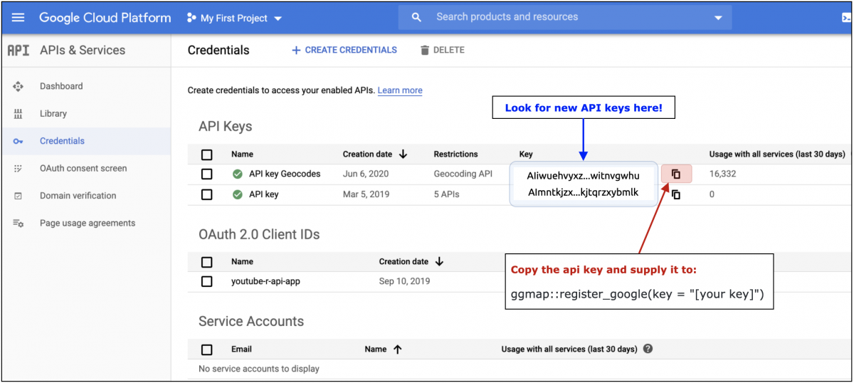
Your private API key needs to be registered with ggmap::register_google(key = "[your key]"). More detailed instructions have been pasted below from the package Github page:
Inside R, after loading the new version of
ggmap, you’ll need provideggmapwith your API key, a hash value (think string of jibberish) that authenticates you to Google’s servers. This can be done on a temporary basis withregister_google(key = "[your key]")or permanently usingregister_google(key = "[your key]", write = TRUE)(note: this will overwrite your~/.Renvironfile by replacing/adding the relevant line). If you use the former, know that you’ll need to re-do it every time you reset R.
After registering your API key, you’ll have access to the two functions for getting geocodes in ggmap: geocode() and revgeocode().
Create a location column
We need the address items into a new location column:
BeerDataUS <- BeerDataUS %>%
  tidyr::unite(data = .,
               # combine all the location elements
               address, city, state, country,
               # new name for variable
               col = "location",
               # separated by comma
               sep = ", ",
               # keep the old columns
               remove = FALSE)
# check the new variable
BeerDataUS %>%
  dplyr::pull(location) %>%
  utils::head()
#>  [1] "13300 Bothell-Everett Highway #304, Mill Creek, Washington, United States"
#>  [2] "621 Front Street, Mukilteo, Washington, United States"
#>  [3] "1524 West Marine View Drive, Everett, Washington, United States"
#>  [4] "404 South Third Street, Mount Vernon, Washington, United States"
#>  [5] "1150 Filbert Street, Philadelphia, Pennsylvania, United States"
#>  [6] "1812 North 15th Street, Tampa, Florida, United States"
We’ll follow the iteration strategy from Charlotte Wickham’s tutorial on purrr.

Get a geocode for a single element
This will produce the following output:
single_element <- base::sample(x = BeerDataUS$location,
                               size = 1,
                               replace = TRUE)
single_element
ggmap::geocode(location = single_element)
> ggmap::geocode(location = single_element)
Source : https://maps.googleapis.com/maps/api/geocode/json?address=NA,+Stillwater,+Minnesota,+United+States&key=xxx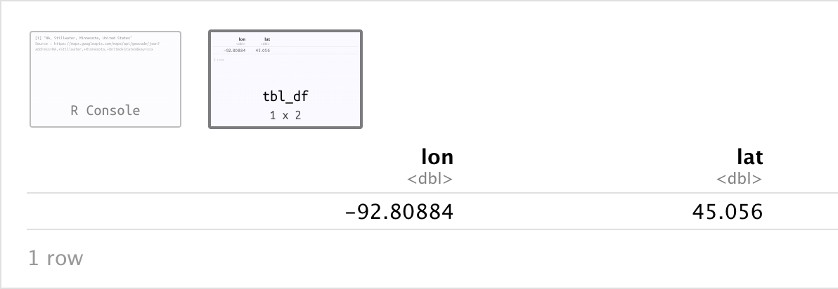
Turn it into a recipe
Now we turn this into a purrr::recipe. We’ll use the purrr::map_df() variant to get the result in a tibble/data.frame.
GeoCoded <- purrr::map_df(.x = BeerDataUS$location, .f = ggmap::geocode)This will take some time, and you should see the following in the console:
When it’s done, you’ll have the following new dataset:
utils::head(x = GeoCoded)
# A tibble: 6 x 2
     lon   lat
   <dbl> <dbl>
1 -122.   47.9
2 -122.   47.9
3 -122.   48.0
4 -122.   48.4
5  -75.2  40.0
6  -82.4  28.0
Now we just need to column bind these to the BeerDataUS dataset and create a new popuptext column. We’ll also rename the lon column as lng because it’s more common in the graphics we’ll be building.
GeoCodedBeerData <- dplyr::bind_cols(BeerDataUS, GeoCoded) %>%
  dplyr::select(
    brewer,
    lng = lon,
    lat,
    dplyr::everything())
# create a popuptext column
GeoCodedBeerData <- GeoCodedBeerData %>%
  dplyr::mutate(popuptext = base::paste0("<b>",
                                 GeoCodedBeerData$brewer,
                                 "</b><br />",
                                 "<i>",
                                 GeoCodedBeerData$address,
                                 ", ",
                                 GeoCodedBeerData$city,
                                 "</i><br />",
                                 "<i>",
                                 GeoCodedBeerData$state,
                                 "</i>"))

utils::head(GeoCodedBeerData)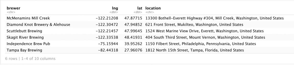
Now that we have a dataset with latitude and longitude columns, we can start mapping the data!
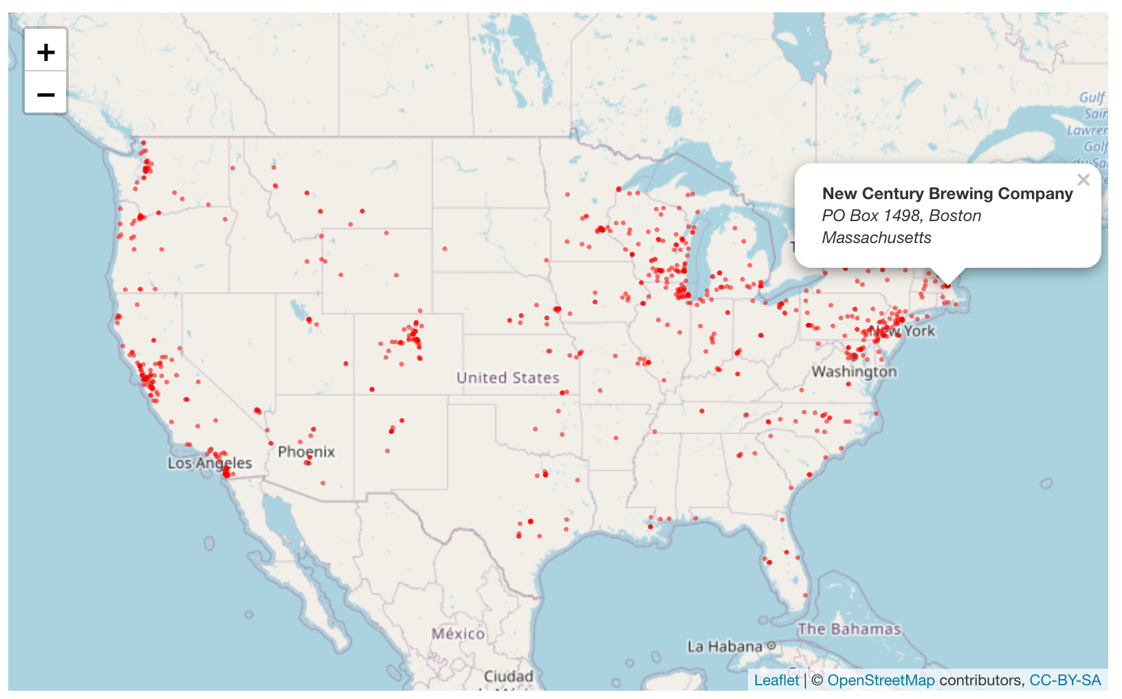
Create a map!
We will use the leaflet package to generate a quick map of brewery locations in the US.
# get a random lat and lng for the setView()
# GeoCodedBeerData %>%
#   dplyr::sample_n(size = 1) %>%
#   dplyr::select(lat, lng)
leaflet::leaflet(data = GeoCodedBeerData) %>%
  leaflet::addTiles() %>%
  leaflet::setView(lng = -96.50923, # random location
                   lat = 39.19729,
                   zoom = 4) %>% # zoom in on US
  leaflet::addCircles(color = "red",
                      lng = ~lng,
                      lat = ~lat,
                      weight = 1.5,
                      popup = ~popuptext)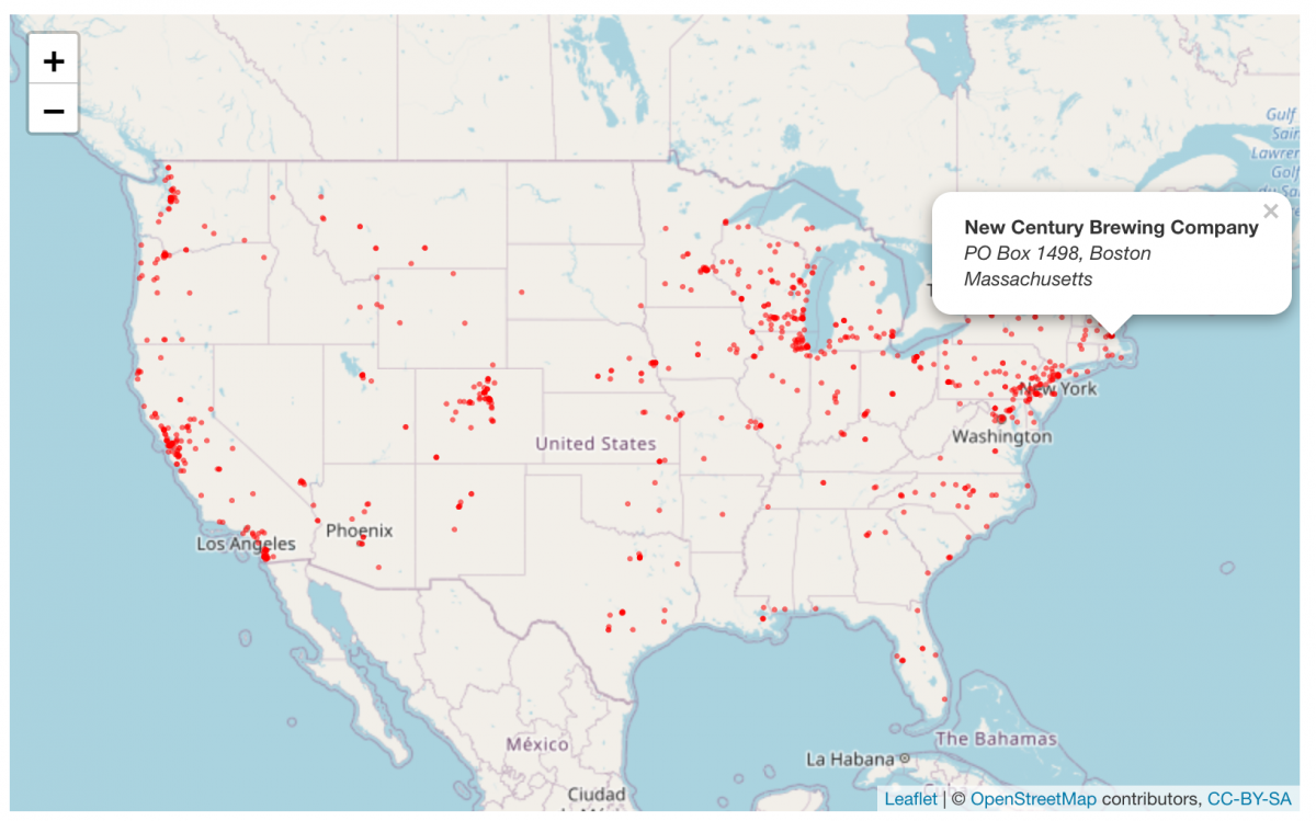
- Getting started with stringr for textual analysis in R - February 8, 2024
- How to calculate a rolling average in R - June 22, 2020
- Update: How to geocode a CSV of addresses in R - June 13, 2020