Many people think of R as a way to visualize data, but it can also be a useful tool to explore datasets and seek possible story ideas.

At the 2023 Investigative Reporters and Editors conference, Charles Minshew, the digital storytelling editor at the Atlanta Journal-Constitution, walked through using basic R code to question datasets. Knowing these techniques can help journalists develop scripts to tackle various datasets.

Packages

In this tutorial, we’ll only be using two R packages. Tidyverse is an R package for data importing, tidying, manipulation and visualization. 

The other package, readxl, is to help R read tabular data from a Microsoft Excel spreadsheet. It is easy to install and can read both .xls format and .xlsx format. Once these are installed, your R will also be equipped with other packages including dplyr and ggplot2.

# to install the packages
# packages.install(tidyverse)
# packages.install(readxl)

Library(tidyverse)
library(readxl)

Data

In order to dig like a true Boston-based reporter, let’s download the Boston government employee earnings report from the city website and see if we can find anything interesting in it.

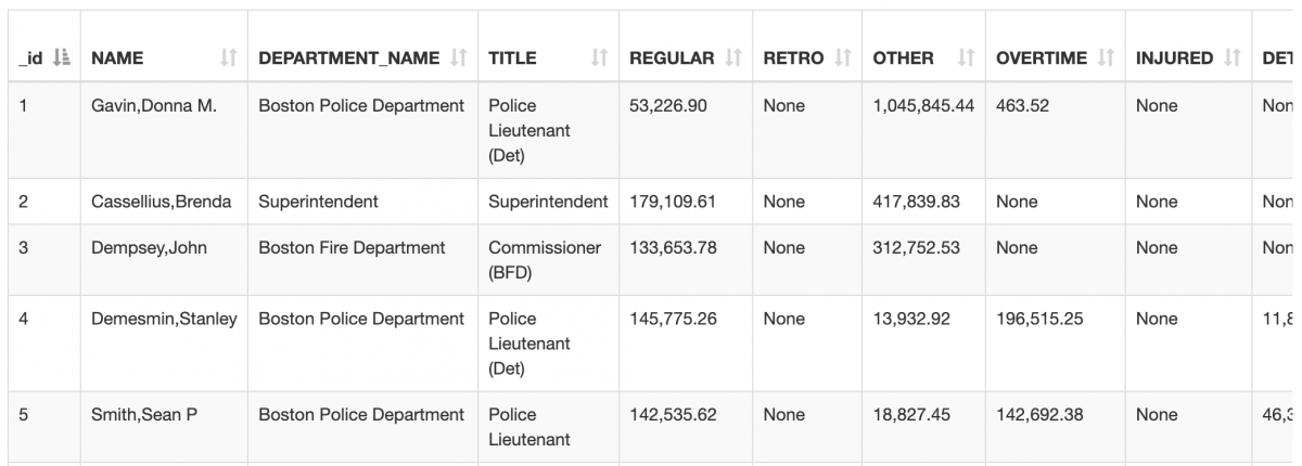
After downloading the dataset, we can put it in a folder next to this R script, rename it as “boston-gov-salaries.xlsx” and load it up in R studio.

salaries <- read_excel("boston-gov-salaries.xlsx", sheet=1)

To start with, we should ask some general questions to know what is going on with this dataset. First things first: what salary-related attributes does this dataset offer?

str(salaries)

After running this code, we can see the following result: name, department name, job title, regular salaries, regular retro earnings (a type of compensation to make up for a compensation shortfall in a previous pay period), overtime earnings, injured earnings and more. 

Note that if any of these attributes confuse you, check the documentation file, which is usually on the same webpage from where you download the data.

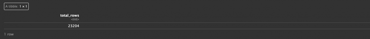
Next, we may want to know how many employees are in this dataset.

salaries %>% summarise(total_rows=n())

%>% means “then” in R. In this line of code, we are trying to say, “Take out the salaries dataset, and then, summarize it by the total row number.” Each row represents one employee record. Hence, the total row number represents the number of employees in this dataset. As shown in the result, a total of 23,204 employees are included in this dataset.

Which departments do they belong to? And which one is the biggest?

salaries %>%
  count(DEPARTMENT_NAME) %>%
  arrange(desc(n))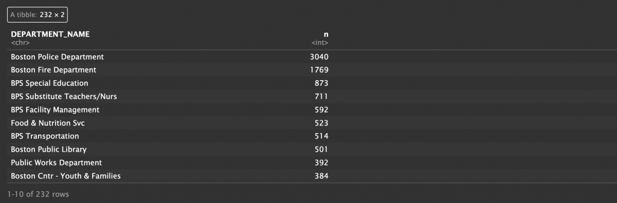

Many people like R because it’s similar to how you might ask a question in your mind. The above code line exactly proves that point. Let’s break it down:

Again, we pull the salaries dataset out.

salaries %>%

Then, we count the department name and add up the counts by the name.

count(DEPARTMENT_NAME) %>%

Then, we arrange the rows by frequencies of department names. desc() allows us to rank them from the most to the least. Without it, the function would rank the data from the least to the most.

arrange(desc(n))

The same logic can also be applied to: how many job titles are included in the dataset. What is the most common one?

salaries %>% 
  count(TITLE) %>% 
  arrange(desc(n))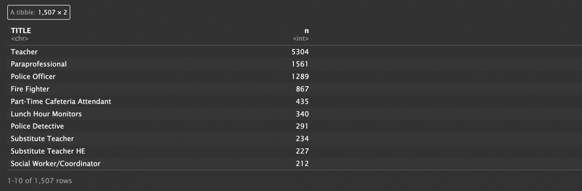

Now, we should have a basic idea about this dataset. We can dig into some descriptive statistics! Such statistics can provide a clear and concise summary of some columns. In our case, these can be useful leads for possible story ideas.

Naturally, we want to see who has the highest salaries.

salaries %>% arrange(desc(TOTAL_GROSS))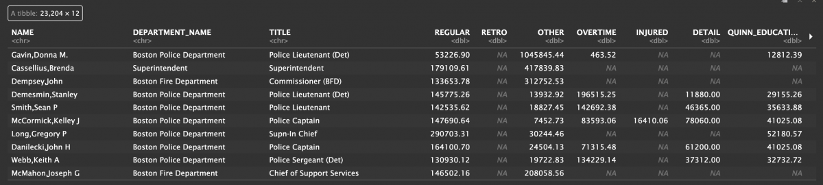

A lot of police department employees are represented here. But I can’t help but notice that, in addition to regular earnings, they also have many other payments. For example, Stanley Demesmin, who has the fourth-highest total, has more overtime than regular earnings. And this leads me to the next question.

Who made the most in overtime payments?

salaries %>% arrange(desc(OVERTIME))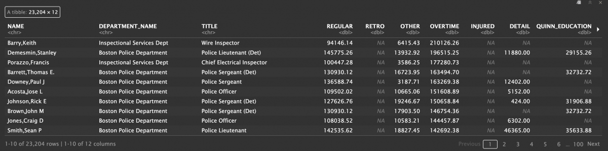

Interesting! Stanley Demesmin doesn’t even have the highest overtime earnings. Keith Barry, who is a wire inspector, made far more in overtime payments. However, because Barry’s regular earnings are not that high, he isn’t one of the top 10 highest earners (he ranks 37th, I checked).

Who made the most while injured? These could lead to some story ideas, as we can follow with what happened to the person with the most injured payments. We can also see if there are any discrepancies between the payments received while employees are out with injuries and what they feel they deserve. It might also raise questions about which injuries are classified as “work-related.”

salaries %>% arrange(desc(INJURED))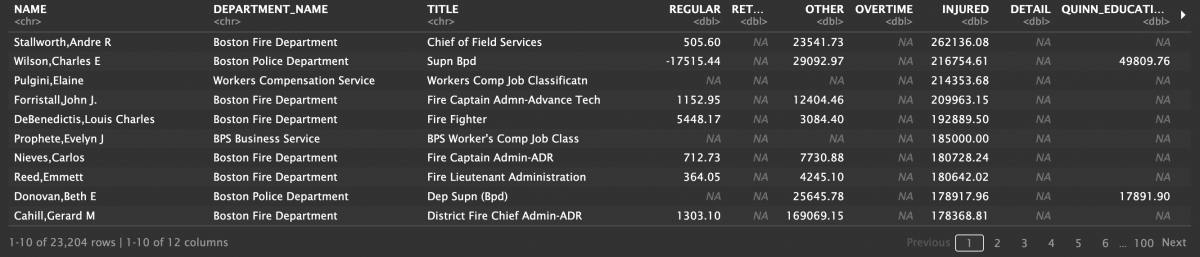

Two names instantly caught my eye — Elaine Pulgini and Evelyn J. Prophete, as they are the only two people on the top injured earnings list who do not belong to the fire or police departments.

After exploring some big-picture ideas, we can dig into some special cases.

For instance, we know that police department employees earned a lot; but how does that compare to other departments? To answer that, we can compare the average total gross earnings among departments.

salaries %>% 
  # group rows by department names
  group_by(DEPARTMENT_NAME) %>% 
  summarise(avg_comp = mean(TOTAL_GROSS)) %>% 
  arrange(desc(avg_comp))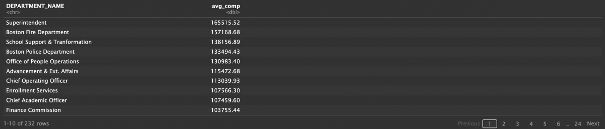

Interesting! It turns out that the average earnings of police department employees are not the highest. Maybe some employees get higher pay just because they are policemen? We can either use the same logic as above to see the salary ranking of titles or we can calculate policemen’s average earnings by doing this: 

salaries %>% 
  # filter rows containing "Police"
  filter(grepl("Police", TITLE)) %>% 
  summarise(avg_pay = mean(TOTAL_GROSS))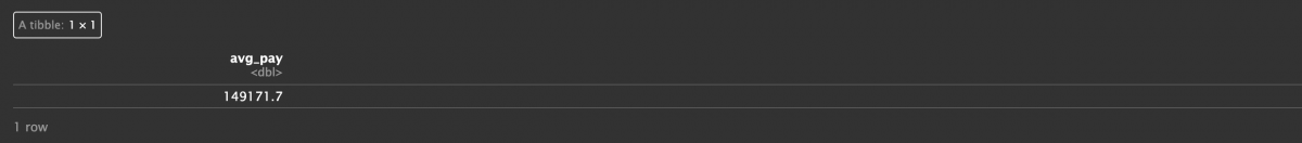

We can also ask if most of the police department employees’ earnings are coming from overtime or injured payments.

# create a dataframe with only police department employees
police<-salaries %>% 
    filter(DEPARTMENT_NAME == "Boston Police Department")

# create a new column with the percentage
police %>%
    select(NAME, TOTAL_GROSS, OVERTIME) %>%
    mutate(overtime_perc = round((OVERTIME / TOTAL_GROSS)*100., digits=2)) %>%
    # we can order the rows by the percentage or by the total revenue, depending on what we want to focus on
    arrange(desc(overtime_perc))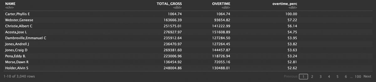

In addition to departments, we can also explore by title, such as who is the highest-paid director? Who is the highest-paid intern? All of these questions can be answered by this line:

salaries %>% 
  filter(grepl("Director", TITLE))

We’ve seen how to use R scripts as part of your pre-reporting process. Once it guides you to some potential story ideas, keep digging for additional facts and reach out to sources. There are many other great datasets on the City of Boston website, as well as many city sites around the country with their own publicly-available datasets. Have fun exploring!

• Author
• Recent Posts

Manyun Zou

Manyun Zou is a graduate student at majoring in applied quantitative analysis and social science at Northeastern University. She was previously a data reporter in China, covering topics like business, gender, and government policies. Her work has also appeared in the Pudding, National Geographic Magazine, and Washingtonian. Manyun is a cat and coffee addict.

Latest posts by Manyun Zou (see all)

• How to use R to dig for story ideas - September 19, 2023