R is a powerful statistical programming language for manipulating, graphing, and modeling data. One of the major positive aspects of R is that it’s open-source (free). But “free” in this case does not necessarily mean “easy.” Learning to program in R is time-consuming and occasionally frustrating, but, fortunately, the number of helpful tools and packages is always growing.

Enter RStudio

RStudio is an integrated development environment (IDE) that streamlines the R programming workflow into an easy to read layout. RStudio also includes useful tools (referred to as packages) for data manipulation (dplyr), cleaning (tidyr), visualizations (ggplot2), report writing (rmarkdown & knitr), and publishing to the web (shiny & ggviz).

Just like R, RStudio is free. They’ve also recently released R Markdown Notebooks, a seamless integration of code, plain text, and results that can be exported into PDF, .docx, or HTML formatted files.

Getting started

Start out by installing R and then RStudio (get the preview version here.)

*If you need help installing R or RStudio, feel free to use  this installation guide.

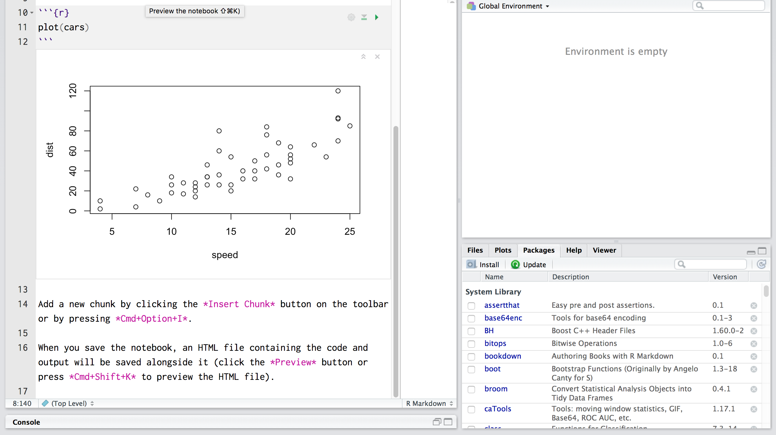
The IDE environment has four panes:

As you can see, the upper-left pane is the editor. The pane in the upper-right, where it says “Environment is empty,” will show the working dataset. The lower-left pane is called the console, which runs the R code. And the pane in the bottom-right will display my results.

Opening a New R Notebook

To get started, click on “File” > “New File” > “R Notebook.“ R Notebooks automatically start off with a title and some sample code, all written in Markdown, a simple markup language. To see how the analysis is woven into the Html, click on the small “Play” arrow button right above “Run Current Chunk”:

This scatterplot will appear:

Save the file (“File” > “Save”) and then click on “Preview” at the top of the pane.

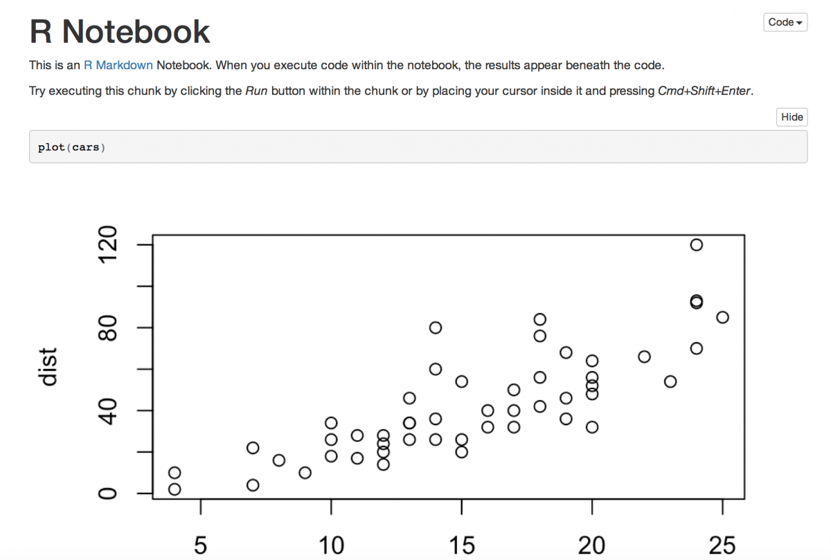
R Notebook, as you can see, can generate an Html preview of your R Notebook file that does a great job of combining markdown text, R code, and results in a clean, crisp, easy-to-share finished product.

Getting started with R: syntax, numbers and text

To get the hang of R, try using RStudio as a simple calculator. Type 2 + 2 directly into the console pane and press enter. You should see this:

[1] 4

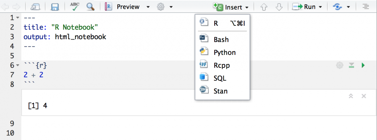
Now, put the same 2 + 2 up in the upper-left editor pane. Notice that all R code must have a ` ` ` {r} before it and a ` ` ` after it. Add that by clicking Insert and “R.”

Next, type in 2 + 2 and click Run and then Run Selected Line(s). Or click Apple-enter. You can add multiple lines and run them all by clicking Run and then Run Current Chunk.

You’re probably hoping to use RStudio for something slightly more advanced than simple arithmetic. Fortunately, R can calculate and store multiple values in variables to reference later. This is done with the <- assignment operator. Type the following and hit enter.

x <- 2 + 2

Notice the a Values table appear in the working dataset – or environment – pane listing x as 4. (The <- is similar to the = sign. In fact, the = sign does the same thing, but the typical convention in R is the <-.)

To see the contents of x , enter it into the console and press enter. You’ll see:

[1] 4

You can also perform mathematical operations with variables. Store 4 + 4 in a variable called y and add it the variable x

y <- 4 + 4
y + x

[1] 12

R identifies numbers and text – or “string” – characters. Text can also be stored into variables using the <- symbol and quotations.

a <- "human"
b <- "error"

Notice, as you add more values to your dataset, they’ll appear in the upper-right pane: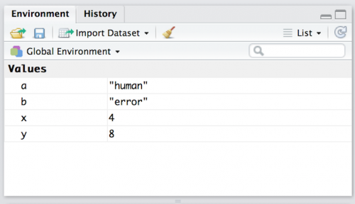

Manipulating strings in R

Text strings are stored differently than numerical data in R. The commands used to manipulate strings are also slightly different.

If you want to combine two strings, use the paste function:

paste(a,b)

[1] "human error"

Objects and data structures in R

R is an object oriented programming language, which means it recognizes objects according to their structure and type. The most common objects in R are atomic vectors and lists.

Atomic Vectors 1.1: numeric and integer vectors

Numeric vectors include “real” numbers with decimal places, while integers are whole numbers. To create numeric vectors, use the command c() which stands for concatenating (a term for combining that you may know from Excel).

Below is an example of a numeric vector of odd numbers less than 10:

odd_vect <- c(1.3, 3.3, 5.5, 7.7, 9.9)

This statement is saying, “combine these five numbers into a vector and call it odd_vect”

If I want to create an integer (or whole number) vector, I need to follow each number with an L

The assignment operator also works in the other direction. Use it to create another numeric vector named even_vect of even integers less than or equal to 10.

c(2L, 4L, 6L, 8L, 10L) -> even_vect

The c() function works for combining separate numerical vectors, too.  Add these two variables together into a new vector called ten_vect and print the contents:

ten_vect <- c(odd_vect, even_vect)

ten_vect

[1] 1.3 3.5 5.1 7.7 9.1 2.0 4.0 6.0 8.0 10.0

The final numeric vector (ten_vect) has combined both the odd and even values into a single vector. See it in the upper-right working dataset pane.

Atomic vectors 1.2: logical and character vectors

Logical vectors return two possible values, TRUE or FALSE. We can use logic to interrogate vectors in order to discover their type.

For example, we can use is.numeric to figure out if the ten_vect vector we created ended up being numeric or integer.

is.numeric(ten_vect)

[1] TRUE

Why did the combination of a numerical and integer vector end up being numeric? This is referred to as coercion. When a less flexible data type (numeric) is combined with a more flexible data type (integer), the more flexible element is coerced into the less flexible type.

Atomic vector 1.3: character vectors

In R, character vectors contain text strings. We can use character vectors to construct a sentence using a combination of c() and <- functions.
We will start with a preposition:

prep_vect <- c("In")

then include a noun

noun_vect <- c("the Brothers Karamazov,")

throw in a subject,

sub_vect <- c("Dmitri")

sprinkle in a verb,

verb_vect <- c("kills")

and finish with an object

obj_vect <- c("his father")

Sentence construction can be a great way to learn how vector objects are structured in R. Atomic vectors are always flat, so you can nest them all…

sent_vect <- c("In",c("the Brothers Karamazov,",c("Dmitri",c("kills",c("his father")))))

sent_vect

[1] "In"                      "the Brothers Karamazov," "Dmitri"                 
[4] "kills"                   "his father"

Or enter them directly:
c("In","the Brothers Karamazov", "Dmitri", "kills", "his father"

[1] "In"                      "the Brothers Karamazov," "Dmitri"                 
[4] "kills"                   "his father"

Both return the same result.

Finally, we can combine each part of the sentence together using  paste:

sent_vect <- paste(prep_vect, noun_vect, sub_vect, verb_vect, obj_vect)


sent_vect
[1] "In the Brothers Karamazov, Dmitri kills his father"

Lists

Unlike vectors – which only contain elements of a single type – lists can contain elements of different types.

We will create a list that includes an integer vector (even_vect) a logical vector (TRUE, FALSE), a full sentence (sent_vect), and a numeric vector (odd_vect) and we will call it my_list

my_list <- list(even_vect, c(TRUE, FALSE), c(sent_vect), c(odd_vect))

We will look at the structure of our list using str

str(my_list)

List of 4
 $ : int [1:5] 2 4 6 8 10
 $ : logi [1:2] TRUE FALSE
 $ : chr "In the Brothers Karamazov, Dmitri kills his father"
 $ : num [1:5] 1.3 3.3 5.5 7.7 9.9

Lists can even contain other lists.

lists_on <- list(list(list(list())))

str(lists_on)

List of 1
 $ :List of 1
 ..$ :List of 1
 .. ..$ : list()

This feature separates Lists from the Atomic vectors described above.

So there you have it! This how-to should give you some basics in R programming. You can save it as HTML, pdf, or Docx file for future reference.

Here’s an R Notebook file for this tutorial.