
Pivoting data from columns to rows (and back!) in the tidyverse
TLDR: This tutorial was prompted by the recent changes to the tidyr package (see the tweet from Hadley Wickham below). Two functions for reshaping columns and rows (gather() and spread()) were replaced with tidyr::pivot_longer() and tidyr::pivot_wider() functions.
Thanks to all 2649 (!!!) people who completed my survey about table shapes! I’ve done analysed the data at https://t.co/hyu1o91xRm and the new functions will be called pivot_longer() and pivot_wider() #rstats— Hadley Wickham (@hadleywickham) March 24, 2019
Load packages
# this will require the newest version of tidyr from github
# devtools::install_github("tidyverse/tidyr")
library(tidyverse)
library(here)
Objectives
This tutorial will cover three concepts about working with data in the tidyverse:
1) tidy data,
2) grouping, and
3) the new pivoting verbs in tidyr
A solid understanding of these topics makes it easier to manipulate and re-structure your data for visualizations and modeling in the tidyverse.
I’ll be using examples of spreadsheets that were designed for data entry, not necessarily statistical modeling or graphics.
My goal is that by showing the reasoning behind the data entry process, you’ll walk away with a better understanding (and hopefully a little less frustration) for why data are collected in so many different ways. To follow along with this tutorial, download the data here.
Part one: Tidy data
Tidy data is… “a standardized way to link the structure of a dataset (its physical layout) with its semantics (its meaning)”
If you’ve worked with SQL and relational databases, you’ll recognize most of these concepts. Hadley Wickham distilled a lot of the technical jargon from Edgar F. Codd’s ‘normal form’ and applied it to statistical terms. More importantly, he translated these essential principles into concepts and terms a broader audience can grasp and use for data manipulation.
# load data from Github
base::load(file = "data/tidyr-data.RData")
The tidy data principles
Tidy data refers to ‘rectangular’ data. These are the data we typically see in spreadsheet software like Googlesheets, Microsoft Excel, or in a relational database like MySQL, PostgreSQL, or Microsoft Access, The three principles for tidy data are:
- Variables make up the columns
- Observations (or cases) go in the rows
- Values are in cells
Put them together, and these three statements make up the contents in a tidy data frame or tibble. While these principles might seem obvious at first, many of the data arrangements we encounter in real life don’t adhere to this guidance.
Indexed vs. Cartesian
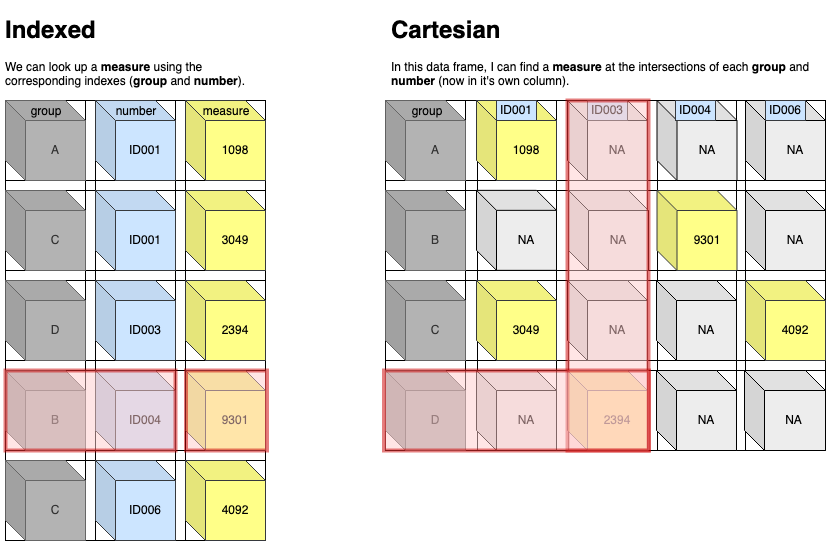
I prefer to refer to tidy data as “indexed”, and wide data as “Cartesian” (this terminology is from the ggplot2 text) because these terms help me understand what is happening when the data get transformed. Two examples are below:
Indexed data
In the Indexed data frame, the group and number variables are used to keep track of each unique value of measure.
Indexed
# A tibble: 5 x 3
  group number measure
  <chr> <chr>    <dbl>
1 A     ID001     1098
2 C     ID001     3049
3 D     ID003     2394
4 B     ID004     9301
5 C     ID006     4092
The same data are represented in the Cartesian data frame, but in this table the measure values are at the intersection of group and each ID### (the number from the previous table).
Cartesian
# A tibble: 4 x 5
  group ID001 ID003 ID004 ID006
  <chr> <dbl> <dbl> <dbl> <dbl>
1 A      1098    NA    NA    NA
2 B        NA    NA  9301    NA
3 C      3049    NA    NA  4092
4 D        NA  2394    NA    NA
As you can see, the Cartesian orientation uses up more columns (and
fills in the gaps with missing (NA) values).
Part two: Grouping
Grouping produces summary data tables using functions from the dplyr package. Similar to GROUP BY in SQL, dplyr::group_by() silently groups a data frame (which means we don’t see any changes) and then applies aggregate functions using dplyr::summarize(). Examples of these are mean(), median(), sum(), n(), sd(), etc.
Take the data frame below, DataTibble, which has 5 variables:
group_var– a categorical groupyear– the calendar year the measurements were collectedx_measurementandy_measurement– these are randomly generated numbers-
ordinal_y_var– this is an ordinal variable corresponding to the values iny_measurement(greater than or equal to800is"high"or3, greater than or equal to500and less than750is"med"or2, and less than500is"low"or1).
DataTibble
# A tibble: 8 x 5
  group_var  year x_measurement y_measurement ordinal_y_var
  <chr>     <dbl>         <dbl>         <dbl> <fct>
1 A          2018          11.8          532. med
2 A          2017          28.5          116. low
3 A          2016          49.2          304. low
4 B          2018          87.6          719. med
5 B          2017          11.3          984. high
6 C          2018          15.9          959. high
7 C          2017          63.8          962. high
8 C          2016          96.0          745. med
If I apply dplyr::group_by() to the group_var in DataTibble, I will see no visible result.
DataTibble %>%
    dplyr::group_by(group_var)
# A tibble: 8 x 5
# Groups:   group_var [3]
  group_var  year x_measurement y_measurement ordinal_y_var
  <chr>     <dbl>         <dbl>         <dbl> <fct>
1 A          2018          11.8          532. med
2 A          2017          28.5          116. low
3 A          2016          49.2          304. low
4 B          2018          87.6          719. med
5 B          2017          11.3          984. high
6 C          2018          15.9          959. high
7 C          2017          63.8          962. high
8 C          2016          96.0          745. med
But when I combine dplyr::group_by() with dplyr::summarize(), I can collapse DataTibble into a smaller table by supplying an aggregate function to summarize(). Below I use summarize() to get the mean of x_measurement and y_messurement and n() to get the total number in each group.
DataTibble %>%
  dplyr::group_by(group_var) %>%
  dplyr::summarize(x_mean = mean(x_measurement),
                   y_mean = mean(y_measurement),
                   no = n())
# A tibble: 3 x 4
  group_var x_mean y_mean    no
  <chr>      <dbl>  <dbl> <int>
1 A           29.8   318.     3
2 B           49.4   852.     2
3 C           58.6   889.     3
Grouping can also work with categorical/factor variables. The code below uses dplyr::count() to summarize the number of ordinal_y_var levels per category of group_var
DataTibble %>%
      dplyr::count(group_var, ordinal_y_var)
# A tibble: 6 x 3
  group_var ordinal_y_var     n
  <chr>     <fct>         <int>
1 A         med               1
2 A         low               2
3 B         high              1
4 B         med               1
5 C         high              2
6 C         med               1
This table isn’t as easy to read, because all of the information is oriented vertically. I can move the values of group_var into individual columns to make it easier on the eyes using tidyr::spread()
DataTibble %>%
    dplyr::count(group_var,ordinal_y_var) %>%
    tidyr::spread(key = group_var,value = n)
# A tibble: 3 x 4
  ordinal_y_var     A     B     C
  <fct>         <int> <int> <int>
1 high             NA     1     2
2 med               1     1     1
3 low               2    NA    NA
Notice how this creates a table with different dimensions? This arrangement can quickly be undone with the accompanying tidyr::gather() function.
tidyr::gather() works a lot like the tidyr::spread() function, but also requires us to specify that the missing values should be removed (na.rm = TRUE).
I also added a dplyr::select() statement to arrange these values so they are similar to the table above.
DataTibble %>%
   dplyr::count(group_var, ordinal_y_var) %>%
   tidyr::spread(key = group_var, value = n) %>%
   tidyr::gather(key = group_var, value = "n",
                 -ordinal_y_var, na.rm = TRUE) %>%
   dplyr::select(group_var, ordinal_y_var, n)
# A tibble: 6 x 3
  group_var ordinal_y_var     n
  <chr>     <fct>         <int>
1 A         med               1
2 A         low               2
3 B         high              1
4 B         med               1
5 C         high              2
6 C         med               1
Part three: Pivoting
All this data manipulation brings us to pivoting, the recent additions to the tidyr package. These will be slowly replacing the functions I used above for reshaping data frames, tidyr::gather() and tidyr::spread(). I found it refreshing to learn that I wasn’t the only person struggling to use these functions. Hadley Wickham, the package developer/author, confessed he also struggles when using these functions,
Many people don’t find the names intuitive and find it hard to remember which direction corresponds to spreading and which to gathering. It also seems surprisingly hard to remember the arguments to these functions, meaning that many people (including me!) have to consult the documentation every time.
Decisions like these are examples of why I appreciate the tidyverse, because I can tell a lot of thought gets put into identifying language that accurately capture the users intentions. Knowing how to reshape data is an important skill for any data scientist, and the tidyr::pivot_ functions make restructuring very clear and explicit.
Pivoting == rotating 90˚
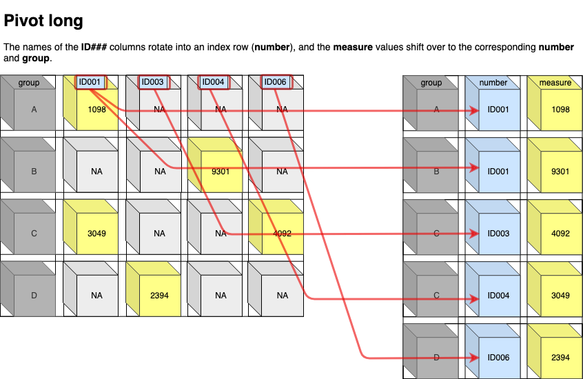
Whenever we use the pivot_ functions, we’re changing angles between the columns and rows. If the tables are pivoting from wide to longer, the column names and values rotate 90˚ into an index row.
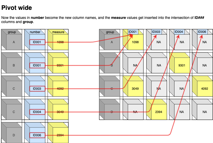
When pivoting from long to wide, the index variable shifts 90˚ across the column names, and the values slide in underneath the names.
These two tidyr::pivot_ functions give users the ability to quickly rotate their data from columns to rows (and back), and provide many arguments for customizing the new data orientations. Tidying data is a great skill to start with because most of the data you’ll encounter in the tidyverse is going to be in columns and rows (or you will want to get them that way).
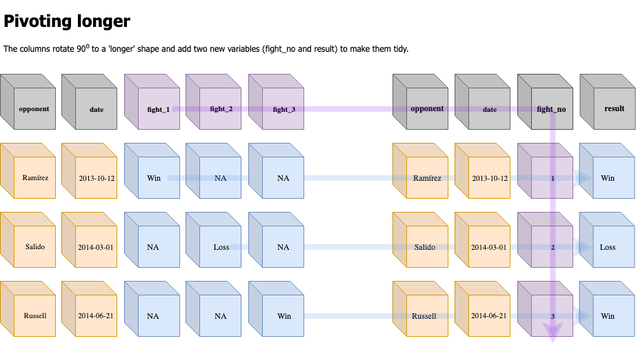
Pivoting Example 1: Categorical/ordinal variable across multiple columns
Vasily Lomachenko, is currently the best pound-for-pound boxer in the world. We’re going to start by manipulating a data set of Lomachenko’s fights from the BoxRec database. The fight information is oriented in a way that makes sense for the person entering the data, but it’s not ideal for analysis or modeling.
LomaWideSmall
opponent       date fight_1 fight_2 fight_3 fight_4 fight_5 fight_6 fight_7 fight_8 fight_9 fight_10 fight_11 fight_12 fight_13 fight_14
1            José Ramírez 2013-10-12     Win    <NA>    <NA>    <NA>    <NA>    <NA>    <NA>    <NA>    <NA>     <NA>     <NA>     <NA>     <NA>     <NA>
2          Orlando Salido 2014-03-01    <NA>    Loss    <NA>    <NA>    <NA>    <NA>    <NA>    <NA>    <NA>     <NA>     <NA>     <NA>     <NA>     <NA>
3        Gary Russell Jr. 2014-06-21    <NA>    <NA>     Win    <NA>    <NA>    <NA>    <NA>    <NA>    <NA>     <NA>     <NA>     <NA>     <NA>     <NA>
4  Chonlatarn Piriyapinyo 2014-11-22    <NA>    <NA>    <NA>     Win    <NA>    <NA>    <NA>    <NA>    <NA>     <NA>     <NA>     <NA>     <NA>     <NA>
5      Gamalier Rodríguez 2015-05-02    <NA>    <NA>    <NA>    <NA>     Win    <NA>    <NA>    <NA>    <NA>     <NA>     <NA>     <NA>     <NA>     <NA>
6         Romulo Koasicha 2015-11-07    <NA>    <NA>    <NA>    <NA>    <NA>     Win    <NA>    <NA>    <NA>     <NA>     <NA>     <NA>     <NA>     <NA>
7          Román Martínez 2016-06-11    <NA>    <NA>    <NA>    <NA>    <NA>    <NA>     Win    <NA>    <NA>     <NA>     <NA>     <NA>     <NA>     <NA>
8        Nicholas Walters 2016-11-26    <NA>    <NA>    <NA>    <NA>    <NA>    <NA>    <NA>     Win    <NA>     <NA>     <NA>     <NA>     <NA>     <NA>
9              Jason Sosa 2017-04-08    <NA>    <NA>    <NA>    <NA>    <NA>    <NA>    <NA>    <NA>     Win     <NA>     <NA>     <NA>     <NA>     <NA>
10        Miguel Marriaga 2017-08-05    <NA>    <NA>    <NA>    <NA>    <NA>    <NA>    <NA>    <NA>    <NA>      Win     <NA>     <NA>     <NA>     <NA>
11   Guillermo Rigondeaux 2017-12-09    <NA>    <NA>    <NA>    <NA>    <NA>    <NA>    <NA>    <NA>    <NA>     <NA>      Win     <NA>     <NA>     <NA>
12          Jorge Linares 2018-05-12    <NA>    <NA>    <NA>    <NA>    <NA>    <NA>    <NA>    <NA>    <NA>     <NA>     <NA>      Win     <NA>     <NA>
13           José Pedraza 2018-12-08    <NA>    <NA>    <NA>    <NA>    <NA>    <NA>    <NA>    <NA>    <NA>     <NA>     <NA>     <NA>      Win     <NA>
14         Anthony Crolla 2019-04-12    <NA>    <NA>    <NA>    <NA>    <NA>    <NA>    <NA>    <NA>    <NA>     <NA>     <NA>     <NA>     <NA>     <NA>
This data arrangement is Cartesian, because each fight number has it’s own column (fight_1 through fight_14), and the result (Win/Loss) is located at the intersection between the fight numbered columns and the corresponding opponent and date. Having the data in this arrangement might seem odd to a data scientist, but this configuration makes sense for a fan entering the fights into a spreadsheet as they happen in real time.
Consider the chronological chain of events involved with a each fight,
- An
opponentis announced, and our excited fan enters the information into the first two column/rows in a spreadsheet and titles it, ‘Lomachenko` - The
datefor the first fight gets entered into theBcolumn (the second in the table), - In order to track an athlete’s win/loss record over the course of their career, a number is also marked for each fight (starting with
1) in a column titled,fight_1. and the result gets put in the corresponding cell (WinorLoss)
As you can see, the steps above are sensible for someone wanting to track a favorite athlete (or sports team) over time. I’ve encountered excel tables with orientations that mirror the sequence of events they’re capturing. This “data-entry friendly” orientation captures enough information to be useful, and it has a few computational abilities. For example, a fan could use filtering to count the number of matches against a particular opponent, or sort the date column to figure what Lomachenko’s late fight. Spreadsheets like these are a cross between a timeline and a record book, and they do a good enough job at both tasks to justify their current structure.
The pivot vignette conveys that ‘wide’ formats or data arrangements are common because their primary purpose and design is centered around recording data (and not visualization or modeling).
Pivoting long
We are going to start by pivoting the LomaWideSmall data frame to a long or ‘tidy’ format. We accomplish this using the tidyr::pivot_longer() function.
LomaWideSmall %>%
   tidyr::pivot_longer(
     cols = starts_with("fight"),
     names_to = "fight_no",
     values_to = "result",
     names_prefix = "fight_",
     na.rm = TRUE)
A tibble: 13 x 4
 opponent               date       fight_no result
  1 José Ramírez           2013-10-12 1        Win
  2 Orlando Salido         2014-03-01 2        Loss
  3 Gary Russell Jr.       2014-06-21 3        Win
  4 Chonlatarn Piriyapinyo 2014-11-22 4        Win
  5 Gamalier Rodríguez     2015-05-02 5        Win
  6 Romulo Koasicha        2015-11-07 6        Win
  7 Román Martínez         2016-06-11 7        Win
  8 Nicholas Walters       2016-11-26 8        Win
  9 Jason Sosa             2017-04-08 9        Win
 10 Miguel Marriaga        2017-08-05 10       Win
 11 Guillermo Rigondeaux   2017-12-09 11       Win
 12 Jorge Linares          2018-05-12 12       Win
 13 José Pedraza           2018-12-08 13       Win
What happens in pivot_longer()?
tidyr::pivot_longer() extends the tidyr::gather() function by adding a few arguments to make this re-structuring more deliberate:
- The
colsargument contains the columns we want to pivot (and it takestidyselecthelper functions). These are going to be the new index columns. - The
names_toandvalues_toare the new columns we will be creating from all of thefight_variables. Thenames_tois the new index column, meaning how would you ‘look up’ the value in an adjacent column. Thevalues_toare the contents of the cells that correspond to each value in thenames_tovariable. - The
names_prefixis a regular expression pattern I can use to clean the old variable names as they become the values in the new columns. I enterfight_here because is will remove the text from the front the variable name and only enter the number into the newfight_novariable.
Unfortunately, we can see that the new fight_no variable is still formatted as a character. Luckily, the new tidyr::pivot_longer() function also has a tidyr::pivot_longer_spec(), which allows for additional specifications on the data transformation.
Pivoting longer (with specifications)
A pivoting
specis a data frame that describes the metadata stored in the column name, with one row for each column, and one column for each variable mashed into the column name.
The tidyr::pivot_longer_spec() function allows even more specifications on what to do with the data during the transformation. Because we are still in the tidyverse, the output is a data fame. Explicitly creating an object that contains data about your data is not necessarily a novel concept in R, but it’s very handy when that object is similar to the other objects you’re already working with (i.e. a data frame or tibble).
Creating a spec for the LomaWideSmall data frame is a three-step process:
1) Define the arguments for reshaping the data
I enter the same arguments I entered above in the tidyr::pivot_longer() function, with the exception of the na.rm = TRUE argument. These results get stored into an object I will name LomaSpec, which is a data frame with three variables in it: .name, .value, and fight_no.
LomaWideSmall %>%
   tidyr::pivot_longer_spec(
      cols = starts_with("fight"),
      names_to = "fight_no",
      values_to = "result",
      names_prefix = "fight_")
LomaSpec
This produces the following (if you’re looking at the output in the R console).
A tibble: 14 x 3
 .name    .value fight_no
  1 fight_1  result 1
  2 fight_2  result 2
  3 fight_3  result 3
  4 fight_4  result 4
  5 fight_5  result 5
  6 fight_6  result 6
  7 fight_7  result 7
  8 fight_8  result 8
  9 fight_9  result 9
 10 fight_10 result 10
 11 fight_11 result 11
 12 fight_12 result 12
 13 fight_13 result 13
 14 fight_14 result 14
The three columns in LomaSpec contain metadata (data about our data) on the transformation I want to perform–specifically the original columns (.name) and the corresponding cell values (.value). The other variable (fight_no) gets carried over from the transformation as well.
2) Format the variable(s) in the spec
If I want to format the fight_no variable, I can include those arguments within the LomaSpec data frame.
# format the variable
 LomaSpec <- LomaSpec %>%
 dplyr::mutate(fight_no = as.numeric(fight_no))
 LomaSpec$fight_no %>% glimpse(78)
# num [1:14] 1 2 3 4 5 6 7 8 9 10 ...
3) Supply the formatted spec object to pivot_longer_spec() function
Now LomaSpec can get supplied to the tidyr::pivot_longer() function and the fight_no variable is properly formatted (note I still need to provide the na.rm = TRUE argument).
# supply it to the pivot_longer
LomaFightsLong %
    tidyr::pivot_longer(spec = LomaSpec,
                        na.rm = TRUE)
LomaFightsLong
# A tibble: 13 x 4
   opponent               date       fight_no result

 1 José Ramírez           2013-10-12        1 Win
 2 Orlando Salido         2014-03-01        2 Loss
 3 Gary Russell Jr.       2014-06-21        3 Win
 4 Chonlatarn Piriyapinyo 2014-11-22        4 Win
 5 Gamalier Rodríguez     2015-05-02        5 Win
 6 Romulo Koasicha        2015-11-07        6 Win
 7 Román Martínez         2016-06-11        7 Win
 8 Nicholas Walters       2016-11-26        8 Win
 9 Jason Sosa             2017-04-08        9 Win
10 Miguel Marriaga        2017-08-05       10 Win
11 Guillermo Rigondeaux   2017-12-09       11 Win
12 Jorge Linares          2018-05-12       12 Win
13 José Pedraza           2018-12-08       13 Win
These data are now in a tidy (indexed) format.
Pivoting wider
It’s less common, but sometimes you’ll need to move variables from a tidy (or indexed) column arrangement into a wide (Cartesian) format.
Pivoting Example 2: Moving categorical or ordinal variables across columns
In order to restructure from a wide to long data frame, we need to use the tidyr::pivot_wider() function. This works much like the pivot_longer() function, but with a few different arguments.
Consider a data frame with the same Lomachenko fight records, but this time arranged by date. Imagine the following events that would lead to the creation of the LomaDatesWide data:
- It’s announced that Lomachenko will be fighting an
opponentandlocationis announced, and our fan enters the information into the first two column/rows in her ‘Lomachenko’ spreadsheet - A
fight_numbercolumn is created to document the number of fights (as they happen) - The date for the first fight (
2013-10-12) gets entered into the the fourth column in the table, and the result (Win) gets put in the corresponding cell - After the scorecards are collected, the
resultis announced (see key below), thefight_recordis updated (with the official outcome of the bout) - The official round and time (
roundsandtime) is recorded for when the fight had to stop (or the total number of rounds if it went the distance), - Titles and belts are listed in the
notessection - When the next fight happens, our fan right-clicks on the last recorded fight, and inserts a new column and date, and repeats steps 1-6
I tend to find tables like these when the data entry is done using ‘Freeze Columns’ or ‘Freeze Rows’.
The LomaFights data frame has Lomachenko’s fight records from his wikipedia table. To create a spreadsheet like the one above, we can use the tidyr::pivot_wider() function.
I add a few dplyr functions to get the data frame to look identical to the excel file above.
LomaFights %>%
    # the columns come from the dates
    tidyr::pivot_wider(names_from = date,
                       # the values will be the result of the fight
                       values_from = result) %>%
    # arrange by the fight number
    dplyr::arrange(no) %>%
    # rearrange the columns
    dplyr::select(opponent, location,
                  dplyr::starts_with("20"),
                  dplyr::everything())
# A tibble: 14 x 22
   opponent   location      `2013-10-12` `2014-03-01` `2014-06-21` `2014-11-22` `2015-05-02` `2015-11-07` `2016-06-11` `2016-11-26` `2017-04-08` `2017-08-05` `2017-12-09` `2018-05-12` `2018-12-08` `2019-04-12`    no record type  rounds time  notes
   <chr>      <chr>         <chr>        <chr>        <chr>        <chr>        <chr>        <chr>        <chr>        <chr>        <chr>        <chr>        <chr>        <chr>        <chr>        <chr>        <int> <chr>  <chr> <chr>  <chr> <chr>
 1 José Ramí… Thomas & Mac… Win          NA           NA           NA           NA           NA           NA           NA           NA           NA           NA           NA           NA           NA               1 1–0    TKO   4 (10) 2:55  Won WBO Int…
 2 Orlando S… Alamodome, S… NA           Loss         NA           NA           NA           NA           NA           NA           NA           NA           NA           NA           NA           NA               2 1–1    SD    12     NA    For vacant …
 3 Gary Russ… StubHub Cent… NA           NA           Win          NA           NA           NA           NA           NA           NA           NA           NA           NA           NA           NA               3 2–1    MD    12     NA    Won vacant …
 4 Chonlatar… Cotai Arena,… NA           NA           NA           Win          NA           NA           NA           NA           NA           NA           NA           NA           NA           NA               4 3–1    UD    12     NA    Retained WB…
 5 Gamalier … MGM Grand Ga… NA           NA           NA           NA           Win          NA           NA           NA           NA           NA           NA           NA           NA           NA               5 4–1    KO    9 (12) 0:50  Retained WB…
 6 Romulo Ko… Thomas & Mac… NA           NA           NA           NA           NA           Win          NA           NA           NA           NA           NA           NA           NA           NA               6 5–1    KO    10 (1… 2:35  Retained WB…
 7 Román Mar… The Theater … NA           NA           NA           NA           NA           NA           Win          NA           NA           NA           NA           NA           NA           NA               7 6–1    KO    5 (12) 1:09  Won WBO jun…
 8 Nicholas … Cosmopolitan… NA           NA           NA           NA           NA           NA           NA           Win          NA           NA           NA           NA           NA           NA               8 7–1    RTD   7 (12) 3:00  Retained WB…
 9 Jason Sosa MGM National… NA           NA           NA           NA           NA           NA           NA           NA           Win          NA           NA           NA           NA           NA               9 8–1    RTD   9 (12) 3:00  Retained WB…
10 Miguel Ma… Microsoft Th… NA           NA           NA           NA           NA           NA           NA           NA           NA           Win          NA           NA           NA           NA              10 9–1    RTD   7 (12) 3:00  Retained WB…
11 Guillermo… The Theater … NA           NA           NA           NA           NA           NA           NA           NA           NA           NA           Win          NA           NA           NA              11 10–1   RTD   6 (12) 3:00  Retained WB…
12 Jorge Lin… Madison Squa… NA           NA           NA           NA           NA           NA           NA           NA           NA           NA           NA           Win          NA           NA              12 11–1   TKO   10 (1… 2:08  Won WBA (Su…
13 José Pedr… Hulu Theater… NA           NA           NA           NA           NA           NA           NA           NA           NA           NA           NA           NA           Win          NA              13 12–1   UD    12     NA    Retained WB…
14 Anthony C… Staples Cent… NA           NA           NA           NA           NA           NA           NA           NA           NA           NA           NA           NA           NA           NA              14 NA     NA    NA     NA    Defending W…
Pivoting wider options
The output is very close to the excel sheet above, except missing values in excel are empty (not an NA like R). I can use the tidyr::pivot_wider(x, values_fill()) to include this change to the data.
LomaFights %>%

    tidyr::pivot_wider(names_from = date,

                       values_from = result,

                       values_fill = list(result = "")) %>%

    dplyr::arrange(no) %>%

    dplyr::select(opponent,

                  location,

                  dplyr::starts_with("20"),
# A tibble: 14 x 16
   opponent            location                                          `2013-10-12` `2014-03-01` `2014-06-21` `2014-11-22` `2015-05-02` `2015-11-07` `2016-06-11` `2016-11-26` `2017-04-08` `2017-08-05` `2017-12-09` `2018-05-12` `2018-12-08` `2019-04-12`
   <chr>               <chr>                                             <chr>        <chr>        <chr>        <chr>        <chr>        <chr>        <chr>        <chr>        <chr>        <chr>        <chr>        <chr>        <chr>        <chr>
 1 José Ramírez        Thomas & Mack Center, Paradise, Nevada, US        Win          ""           ""           ""           ""           ""           ""           ""           ""           ""           ""           ""           ""           ""
 2 Orlando Salido      Alamodome, San Antonio, Texas, US                 ""           Loss         ""           ""           ""           ""           ""           ""           ""           ""           ""           ""           ""           ""
 3 Gary Russell Jr.    StubHub Center, Carson, California, US            ""           ""           Win          ""           ""           ""           ""           ""           ""           ""           ""           ""           ""           ""
 4 Chonlatarn Piriyap… Cotai Arena, Macau, SAR                           ""           ""           ""           Win          ""           ""           ""           ""           ""           ""           ""           ""           ""           ""
 5 Gamalier Rodríguez  MGM Grand Garden Arena, Paradise, Nevada, US      ""           ""           ""           ""           Win          ""           ""           ""           ""           ""           ""           ""           ""           ""
 6 Romulo Koasicha     Thomas & Mack Center, Paradise, Nevada, US        ""           ""           ""           ""           ""           Win          ""           ""           ""           ""           ""           ""           ""           ""
 7 Román Martínez      The Theater at Madison Square Garden, New York C… ""           ""           ""           ""           ""           ""           Win          ""           ""           ""           ""           ""           ""           ""
 8 Nicholas Walters    Cosmopolitan of Las Vegas, Paradise, Nevada, US   ""           ""           ""           ""           ""           ""           ""           Win          ""           ""           ""           ""           ""           ""
 9 Jason Sosa          MGM National Harbor, Oxon Hill, Maryland, US      ""           ""           ""           ""           ""           ""           ""           ""           Win          ""           ""           ""           ""           ""
10 Miguel Marriaga     Microsoft Theater, Los Angeles, California, US    ""           ""           ""           ""           ""           ""           ""           ""           ""           Win          ""           ""           ""           ""
11 Guillermo Rigondea… The Theater at Madison Square Garden, New York C… ""           ""           ""           ""           ""           ""           ""           ""           ""           ""           Win          ""           ""           ""
12 Jorge Linares       Madison Square Garden, New York City, New York, … ""           ""           ""           ""           ""           ""           ""           ""           ""           ""           ""           Win          ""           ""
13 José Pedraza        Hulu Theater, New York City, New York, US         ""           ""           ""           ""           ""           ""           ""           ""           ""           ""           ""           ""           Win          ""
14 Anthony Crolla      Staples Center, Los Angeles, California, US       ""           ""           ""           ""           ""           ""           ""           ""           ""           ""           ""           ""           ""           NA
Another neat part of the pivot_wider() function is the values_from argument can take multiple columns. For example, if I wanted to see how man Wins resulted in TKOs (technical knock-outs) or KOs (knock-outs) and their corresponding rounds and time, I could use the following to see rounds and time in separate columns.
LomaFights %>%

    dplyr::filter(result == "Win") %>%

    pivot_wider(names_from = c(type),

                values_from = c(rounds, time),

                values_fill = list(rounds = "",

                                   time = "")) %>%

    dplyr::select(opponent,

                  dplyr::contains("_KO"),

                  dplyr::contains("_TKO"))
# A tibble: 12 x 5
   opponent               rounds_KO time_KO rounds_TKO time_TKO
   <chr>                  <chr>     <chr>   <chr>      <chr>
 1 José Ramírez           ""        ""      4 (10)     2:55
 2 Gary Russell Jr.       ""        ""      ""         ""
 3 Chonlatarn Piriyapinyo ""        ""      ""         ""
 4 Gamalier Rodríguez     9 (12)    0:50    ""         ""
 5 Romulo Koasicha        10 (12)   2:35    ""         ""
 6 Román Martínez         5 (12)    1:09    ""         ""
 7 Nicholas Walters       ""        ""      ""         ""
 8 Jason Sosa             ""        ""      ""         ""
 9 Miguel Marriaga        ""        ""      ""         ""
10 Guillermo Rigondeaux   ""        ""      ""         ""
11 Jorge Linares          ""        ""      10 (12)    2:08
12 José Pedraza           ""        ""      ""         ""
We can also use the tidyr::pivot_wider() function like tidyr::spread() function above. If I want to see the fight results by type, but with Win and Loss in separate columns, I can use the following sequence.
LomaFights %>%

    dplyr::filter(!is.na(result)) %>%

    dplyr::count(type, result) %>%

    tidyr::pivot_wider(

            names_from = result,

            values_from = n,

            values_fill = list(n = 0))
# A tibble: 6 x 3
  type    Win  Loss
  <chr> <int> <int>
1 KO        3     0
2 MD        1     0
3 RTD       4     0
4 SD        0     1
5 TKO       2     0
6 UD        2     0
As you can see, these new tidyr::pivot_ functions extend tidyr::gather() and tidyr::spread() with more options and flexibility. I think you’ll find these are a welcome addition to the data wrangling packages and in the tidyverse.
Read more
- Check out the pivoting vignette on the tidyverse website.
- Alison Presmanes Hill has some great examples in this Github repo.
- Read the
NEWS.mdfile on thetidyrgithub page for new changes to these functions (and others!) - Be sure to check out Vasiliy Lomachenko when he fights Anthony Crolla on April 12!
- Getting started with stringr for textual analysis in R - February 8, 2024
- How to calculate a rolling average in R - June 22, 2020
- Update: How to geocode a CSV of addresses in R - June 13, 2020


Thanks for your article. It is very helpful. However, your first piece of code for pivot_longer doesn’t work. na.rm = TRUE throws an error and needs to be replaced with values_drop_na = TRUE. This was the only way I could get it to work. Using R 4.0.0.
Great post and it helps to have the equivalence gather/spread with longer/wider. For me it was useful the pivot wider image ‘tracking’ the labels/variables.
How to convert a long year monthly rainfall data from a single column to twelve rows in r code?